Vote Wrapper: Regression

In this tutorial we show how to wrap a simple regression model with Capsa Vote Wrapper. The Vote wrapper predicts epistemic uncertainty, which increases in regions where data is sparse or absent. This differs from aleatoric uncertainty, which increases where the relationship between inputs and outputs is noisy or ambiguous (compare with the sculpt wrapper regression tutorial).

Step 1: Initial Setup

This step is universal and dependant to your specific model and dataset you are using.

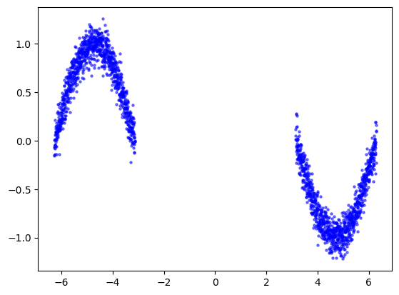
In this example our goal is to estimate a sinusoidal function. We generate synthetic data adding randomness to the function, where the randomness in one area is much larger than the rest, and predict it with a simple neural network.

import torch
import math
import numpy as np
import tqdm
import matplotlib.pyplot as plt

torch.manual_seed(1)
np.random.seed(1)

def fn(x, noise_level = 0.1):
    y = torch.sin(x)
    noise = torch.randn(x.shape)
    y += noise * noise_level
    return y

x_train_left = torch.linspace(-2*math.pi,-math.pi,1000).unsqueeze(-1)
x_train_right = torch.linspace(math.pi,2*math.pi,1000).unsqueeze(-1)
x_train_full = torch.cat([x_train_left, x_train_right], dim=0)
y_train_full = fn(x_train_full)

plt.scatter(x_train_full, y_train_full, label='Ground truth data', s=5, c='blue',alpha=0.5)
plt.show()

In this tutorial we are using a simple sequential model.

from torch import nn

model = nn.Sequential(nn.Linear(1, 64),
            nn.ReLU(),
            nn.Linear(64, 64),
            nn.ReLU(),
            nn.Linear(64, 64),
            nn.ReLU(),
            nn.Linear(64, 1))

Step 2: Wrapping the model

Using Capsa requires constructing a wrapper and applying it to your model. This wrapper adds new outputs and parameters to the model, which will be trained in the following step.

from capsa_torch import vote

#Wrap model with vote wrapper
wrapper = vote.Wrapper(n_voters=4, weight_noise=0.4)
wrapped_model = wrapper(model)

Note

The vote-wrapped model will not produce useful outputs unless it is first trained or finetuned, as seen in the following step. Read the wrapper documentation for more details.

Step 3: Training

from sklearn.model_selection import train_test_split

opt = torch.optim.Adam(wrapped_model.parameters(), lr=1e-3)
loss_func = torch.nn.MSELoss(reduction='mean')

x_train, x_val, y_train, y_val = train_test_split(x_train_full.numpy(), y_train_full.numpy(), test_size=0.2, random_state=42)
x_train, x_val, y_train, y_val = torch.from_numpy(x_train), torch.from_numpy(x_val), torch.from_numpy(y_train), torch.from_numpy(y_val)

prog_bar = tqdm.trange(500)
for t in prog_bar:
    #The model now returns 2 outputs (when return_risk=True)
    y_pred = wrapped_model(x_train, training=True)
    # Use the loss term for your distribution
    loss = loss_func(y_train, y_pred)

    opt.zero_grad()
    loss.backward()
    opt.step()
    
    prog_bar.set_postfix(loss = loss.item())

100%|██████████| 500/500 [00:07<00:00, 62.54it/s, loss=0.0109] 

Step 4: Testing & Evaluation

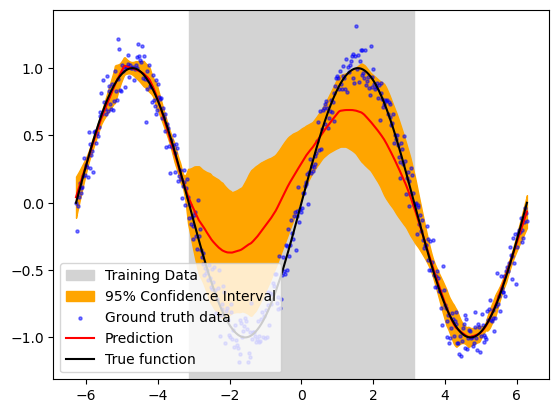
Once you have trained your wrapped model, you will get a risk value for every output to your model if return_risk = True. Here, you can visualize the predicted risk as the orange filling area in the plot.

#Generate testing data
x_test = torch.linspace(-2*math.pi,2*math.pi,500).unsqueeze(-1)
y_test_noisy = fn(x_test)
y_test_true = fn(x_test, noise_level = 0.0)

with torch.no_grad():
    y_pred_test, risk_test = wrapped_model(x_test, return_risk = True)
ln2 = plt.axvspan(-torch.pi, torch.pi, color='lightgray', label='Training Data')
plt.fill_between(x_test.ravel(), y_pred_test.detach().ravel()+3*risk_test.ravel(),y_pred_test.detach().ravel()-3*risk_test.ravel(),color='orange',alpha=1, label='95% Confidence Interval')
plt.scatter(x_test, y_test_noisy, label='Ground truth data', s=5, c='blue',alpha=0.5)
plt.plot(x_test, y_pred_test.detach(), label='Prediction', c='red')
plt.plot(x_test, y_test_true, label='True function', c='black')
plt.legend(loc='best')

<matplotlib.legend.Legend at 0x7fceb018c310>

Epistemic Uncertainty Calibration

We can also compare the ground truth errors with the epistemic risk score

gt_error = torch.abs(y_test_true - y_pred_test.detach())

plt.figure()
ax = plt.gca()
plt.ylabel('Epistemic Uncertainty')
ln2 = ax.axvspan(-torch.pi, torch.pi, color='lightgray', label='Training Data')
ln1 = ax.plot(x_test, risk_test, label='Epistemic Uncertainty', c='green')
ax2 = plt.twinx()
ln3 = ax2.plot(x_test, gt_error, label='Ground Truth Error', c='red')
plt.ylabel('Ground Truth Error')
lns = ln1+[ln2]+ln3
labs = [l.get_label() for l in lns]
ax.legend(lns, labs, loc='upper right')
plt.show()

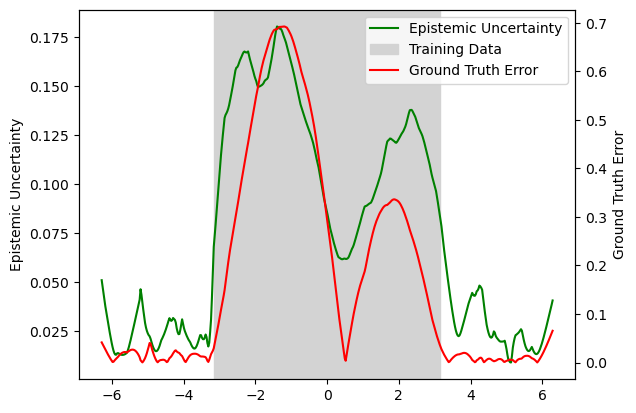
Epistemic uncertainty is generally less well calibrated than aleatoric uncertainty, as illustrated in the sculpt wrapper regression tutorial. Aleatoric uncertainty can be learned and calibrated directly from the training data, whereas epistemic uncertainty reflects gaps in the model’s knowledge caused by insufficient training data coverage.

Model calibration can be improved by adjusting parameters such as weight_noise and n_voters. In most real-world scenarios, gaps in the training data are less severe, and the default vote wrapper parameters are typically sufficient.

Calibration can be visualized using the regression_calibration_curve function from the themis_utils calibration toolkit, where perfect calibration corresponds to the diagonal line y = x.

!pip install -q themis-utils[calib]

from themis_utils.calibration import regression_calibration_curve

exp_conf, obs_conf = regression_calibration_curve(y_test_noisy.squeeze().numpy(), y_pred_test.detach().squeeze().numpy(), risk_test.squeeze().numpy(), num_samples=10)

plt.figure()
ax = plt.gca()
ax.plot(exp_conf, obs_conf, label='Calibration Curve')
ax.plot([0, 1], [0, 1], '--', color='black', label='Perfect Calibration')
plt.xlabel('Confidence Quantile')
plt.ylabel('Fraction Within Confidence Quantile')
plt.xlim([0, 1])
plt.ylim([0, 1])
ax.legend()
plt.show()

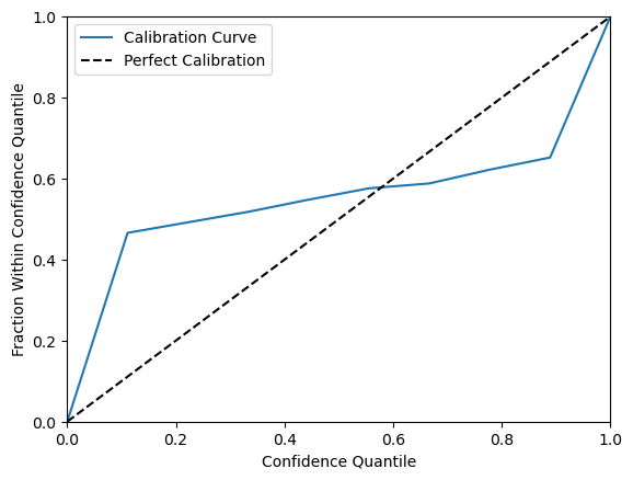
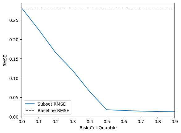
Although this calibration is weaker than the one in the sculpt wrapper regression tutorial, the key point is that epistemic uncertainty provides a strong signal for distinguishing well-supported predictions from weaker, extrapolated ones. This can be evaluated using a risk-cut plot, which reports the RMSE (root mean square error) of the retained predictions after sequentially removing the highest-risk predictions across quantiles.

from capsa_torch.interpret import RegressionMetrics, top_percent_risk_cut_metric

quantiles, metrics = top_percent_risk_cut_metric(y_pred_test.squeeze(), 
                                                 risk_test.squeeze(), 
                                                 y_test_true.squeeze(), 
                                                 10, 
                                                 metric_fn=RegressionMetrics.rmse)

errors = y_pred_test - y_test_true
sq_errors = torch.square(errors)
rmse = torch.sqrt(torch.mean(sq_errors))

plt.figure()
plt.plot(quantiles, metrics, label='Subset RMSE')
plt.axhline(rmse, color='black', linestyle='--', label=f'Baseline RMSE')
plt.xlabel('Risk Cut Quantile')
plt.ylabel('RMSE')
plt.xlim(0, 0.9)
plt.ylim(0, None)
plt.legend()
plt.show()

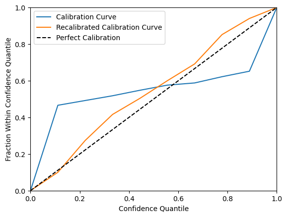
If a stronger risk calibration would be beneficial to your use case, you can use the recalibrate_regression function from the themis_utils.calibration package. Note that as this simply scales the risk values, it will not change the quality of the risk-cut plot. You can see an example of risk calibration below.

from themis_utils.calibration import recalibrate_regression

x_val = torch.linspace(-2*math.pi,2*math.pi,500).unsqueeze(-1)
y_val_noisy = fn(x_val)
y_pred_val, risk_val = wrapped_model(x_val, return_risk=True)

scale = recalibrate_regression(y_val_noisy.detach().squeeze(), y_pred_val.detach().squeeze(), risk_val.detach().squeeze(), num_samples=10)
risk_calibrated = scale * risk_test
print('Scale: ', scale)

exp_conf_recal, obs_conf_recal = regression_calibration_curve(y_test_noisy.squeeze().numpy(), y_pred_test.detach().squeeze().numpy(), risk_calibrated.squeeze().numpy(), num_samples=10)

plt.figure()
ax = plt.gca()
ax.plot(exp_conf, obs_conf, label='Calibration Curve')
ax.plot(exp_conf_recal, obs_conf_recal, label='Recalibrated Calibration Curve')
ax.plot([0, 1], [0, 1], '--', color='black', label='Perfect Calibration')
plt.xlabel('Confidence Quantile')
plt.ylabel('Fraction Within Confidence Quantile')
plt.xlim([0, 1])
plt.ylim([0, 1])
ax.legend()
plt.show()

Scale:  3.8814635113760416