Sculpt Wrapper: Depth Estimation with U-Net

In this tutorial, we show how to wrap a U-Net model using a Sculpt wrapper and train it on the task of monocular end-to-end depth estimation using the “NYU Depth V2” dataset (RGB-to-depth image pairs of indoor scenes). Specifically, the model’s final layer outputs a single H × W activation map. The U-Net model is a type of convolutional neural network (CNN) whose structure resembles the letter “U”.

After wrapping, we can output both the depth of single scenes and the uncertainty of depth estimation over the images.

Step 1: Initial Setup

import h5py
import torch
import time
import numpy as np
import matplotlib.pyplot as plt
from tqdm import tqdm
import torch.nn as nn
from torch.nn import functional as F
from torch.utils.data import DataLoader
import lightning.pytorch as pl
from lightning.pytorch.callbacks import ModelCheckpoint

DEVICE = "cuda" if torch.cuda.is_available() else "cpu"
PIN_MEMORY = True if DEVICE == "cuda" else False
BS = 128
EP = 200
LR = 3e-5
IMAGE_HEIGHT = 64
IMAGE_WIDTH = 80

Functions for loading the “NYU Depth V2” dataset

def _load_depth_data(id_path):
    data = h5py.File(id_path, "r")
    # (8192, 128, 160, 3), (8192, 128, 160, 1)
    train_x, train_y = data["x"], data["y"]
    # (256, 128, 160, 3), (256, 128, 160, 1)
    test_x, test_y = data["x_test"], data["y_test"]
    return (train_x, train_y), (test_x, test_y)


def _totensor_and_normalize(xy_pair):
    x, y = xy_pair
    x, y = np.array(x), np.array(y)
    x = torch.tensor(x)
    y = torch.tensor(y)
    return x / 255.0, y / 255.0


def _get_normalized_ds(x, y, shuffle=True):
    x, y = _totensor_and_normalize((x, y))
    x = torch.permute(x, (0, 3, 1, 2))
    x = F.interpolate(x, scale_factor=0.5, mode='nearest')
    y = torch.permute(y, (0, 3, 1, 2))
    y = F.interpolate(y, scale_factor=0.5, mode='nearest')
    ds = torch.utils.data.TensorDataset(x, y)
    return ds


def get_datasets(id_path, ood_path=None):
    (x_train, y_train), (x_test, y_test) = _load_depth_data(id_path)
    ds_train = _get_normalized_ds(x_train, y_train)
    ds_test = _get_normalized_ds(x_test, y_test)
    return ds_train, ds_test

Download the Dataset

You’ll need to download the dataset from Google drive.

Google drive link: https://drive.google.com/file/d/1g5TEJXxDR3xTXr8zZ0zR8xaxGE55DOdR/view?usp=sharing (660 MB)

Note: to keep this tutorial short we use a small subset of the original dataset and reduce the image resolution
Original(approx): 440GB, 40000 frames, 480x640
Reduced(approx): 660MB, 8000 frames, 128x160

To improve model performance further, please train on the full dataset: https://cs.nyu.edu/~silberman/datasets/nyu_depth_v2.html

ds_train, ds_test = get_datasets(
    id_path = "nyu.h5",
)

# create the training and test data loaders
trainLoader = DataLoader(ds_train, shuffle=True,
	batch_size=BS, pin_memory=True, num_workers=4)
testLoader = DataLoader(ds_test, shuffle=False,
	batch_size=BS, pin_memory=True, num_workers=4)

Creating the base U-Net model

class conv_block(nn.Module):
    def __init__(self, in_c, out_c):
        super().__init__()
        self.conv1 = nn.Conv2d(in_c, out_c, kernel_size=3, padding=1)
        self.bn1 = nn.BatchNorm2d(out_c, track_running_stats = False)
        self.conv2 = nn.Conv2d(out_c, out_c, kernel_size=3, padding=1)
        self.bn2 = nn.BatchNorm2d(out_c, track_running_stats = False)
        self.relu = nn.ReLU()
    def forward(self, inputs):
        x = self.conv1(inputs)
        x = self.bn1(x)
        x = self.relu(x)
        x = self.conv2(x)
        x = self.bn2(x)
        x = self.relu(x)
        return x

class encoder_block(nn.Module):
    def __init__(self, in_c, out_c):
        super().__init__()
        self.conv = conv_block(in_c, out_c)
        self.pool = nn.MaxPool2d((2, 2))
    def forward(self, inputs):
        x = self.conv(inputs)
        p = self.pool(x)
        return x, p

class decoder_block(nn.Module):
    def __init__(self, in_c, out_c):
        super().__init__()
        self.up = nn.ConvTranspose2d(in_c, out_c, kernel_size=2, stride=2, padding=0)
        self.conv = conv_block(out_c+out_c, out_c)
    def forward(self, inputs, skip):
        x = self.up(inputs)
        x = torch.cat([x, skip], axis=1)
        x = self.conv(x)
        return x

class build_unet(nn.Module):
    def __init__(self):
        super().__init__()
        """ Encoder """
        self.e1 = encoder_block(3, 64)
        self.e2 = encoder_block(64, 128)
        self.e3 = encoder_block(128, 256)
        self.e4 = encoder_block(256, 512)
        """ Bottleneck """
        self.b = conv_block(512, 1024)
        """ Decoder """
        self.d1 = decoder_block(1024, 512)
        self.d2 = decoder_block(512, 256)
        self.d3 = decoder_block(256, 128)
        self.d4 = decoder_block(128, 64)
        """ Classifier """
        self.outputs = nn.Conv2d(64, 1, kernel_size=1, padding=0)
    def forward(self, inputs):
        """ Encoder """
        s1, p1 = self.e1(inputs)
        s2, p2 = self.e2(p1)
        s3, p3 = self.e3(p2)
        s4, p4 = self.e4(p3)
        """ Bottleneck """
        b = self.b(p4)
        """ Decoder """
        d1 = self.d1(b, s4)
        d2 = self.d2(d1, s3)
        d3 = self.d3(d2, s2)
        d4 = self.d4(d3, s1)
        """ Classifier """
        outputs = self.outputs(d4)
        return outputs

Step 2: Wrapping the model

In order to wrap your model, you need to pass in the model along with a sample input to your model.

from capsa_torch import sculpt

unet = build_unet().to(DEVICE)

dist = sculpt.Normal
model = sculpt.Wrapper(dist, n_layers = 3)(unet)

Step 3: Training the model

For the Sculpt wrapper, we need to add our risk loss to the original loss when training. We can use the dist.loss_function provided in the sculpt module.

Here we use pytorch_lightning to simplify the training process. We create a LightningModel object that wraps our model and implements the training/validation step logic

class LightningModel(pl.LightningModule):
    def __init__(self, model, lr, orig_loss_mul=10) -> None:
        super().__init__()
        self.model = model
        self.orig_loss_fn = torch.nn.MSELoss()
        self.lr = lr
        self.orig_loss_mul = orig_loss_mul
        self.save_hyperparameters(ignore=["model"])
    
    def forward(self, *args, **kwargs):
        return self.model(*args, **kwargs)

    def training_step(self, batch, batch_idx):
        x, y = batch
        pred, risk = self.model(x, return_risk=True)
        risk_loss = dist.loss_function(y, pred, risk)
        orig_loss = self.orig_loss_fn(pred, y)
        loss = risk_loss + self.orig_loss_mul * orig_loss
        self.log_dict({"train_loss": loss, "train_risk_loss":risk_loss, "train_orig_loss": orig_loss}, prog_bar=True)
        return loss

    def validation_step(self, batch, batch_idx):
        x, y = batch
        pred, risk = self.model(x, return_risk=True)
        risk_loss = dist.loss_function(y, pred, risk)
        orig_loss = self.orig_loss_fn(pred, y)
        loss = risk_loss + self.orig_loss_mul * orig_loss
        self.log_dict({"val_loss": loss, "val_risk_loss":risk_loss, "val_orig_loss": orig_loss}, prog_bar=True)
        return loss
    
    def configure_optimizers(self):
        return torch.optim.Adam(model.parameters(), lr=self.lr)

Note: Use (tensorboard --logdir lightning_logs) to monitor training progress

# Load the best model from checkpoint
pl_model = LightningModel.load_from_checkpoint('lightning_logs/version_0/checkpoints/epoch=37-step=2432.ckpt', model=model, lr=LR)
model = pl_model.model # Extract the model from the lightning wrapper

pl_model = LightningModel(model, LR)
trainer = pl.Trainer(max_epochs=EP, callbacks=[ModelCheckpoint(monitor="val_loss")]) # Save best val loss model
trainer.fit(pl_model, train_dataloaders=trainLoader, val_dataloaders=testLoader)

Step 4: Testing & Evaluation

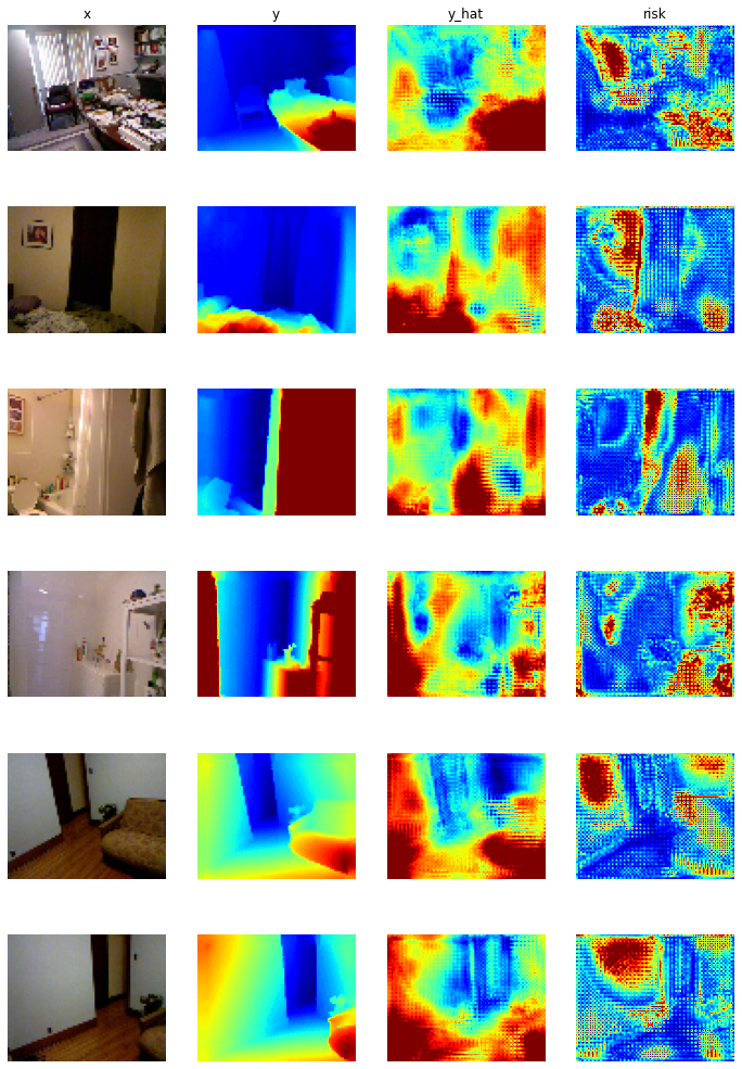
Once you have trained your wrapped model, you will get a WxH array of risk values for every activation map output to your model.

def visualize_depth_map(model, ds_or_tuple, name="", vis_path=None, plot_risk=True):
    model.eval()
    model.to(DEVICE)
    col = 4 if plot_risk else 3
    fgsize = (12, 18) if plot_risk else (8, 14)
    fig, ax = plt.subplots(6, col, figsize=fgsize)  # (5, 10)
    fig.suptitle(name, fontsize=16, y=0.92, x=0.5)

    perm = torch.randperm(len(ds_or_tuple))
    for i in range(6):
        x, y = ds_or_tuple[perm[i]]
        x = x[None].to(DEVICE)
        
        if plot_risk:
            y_hat, risk = model(x, return_risk=True)
            x, y, y_hat, risk = x[0], y[0], y_hat[0], risk[0]
        else:
            y_hat = model(x)
            x, y, y_hat = x[0], y[0], y_hat[0]
            
        x = np.transpose(x.cpu().detach().numpy(), (1, 2, 0))
        y = y.cpu().detach().numpy()

        ax[i, 0].imshow(x)
        ax[i, 1].imshow(y, cmap=plt.cm.jet)
        ax[i, 2].imshow(
            (torch.clamp(y_hat[0], min=0, max=1)).cpu().detach().numpy(),
            cmap=plt.cm.jet,
        )
        if plot_risk:
            ax[i, 3].imshow(
                (torch.clamp(risk[0], min=0, max=1)).cpu().detach().numpy(),
                cmap=plt.cm.jet,
            )

    # name columns
    ax[0, 0].set_title("x")
    ax[0, 1].set_title("y")
    ax[0, 2].set_title("y_hat")
    if plot_risk:
        ax[0, 3].set_title("risk")

    # turn off axis
    [ax.set_axis_off() for ax in ax.ravel()]

    if vis_path != None:
        plt.savefig(f"{vis_path}/{name}.pdf", bbox_inches="tight", format="pdf")
        plt.close()
    else:
        plt.show()

visualize_depth_map(model, ds_test, plot_risk=True)

We can plot a calibration curve using the output predictions and risks from the Sculpt Wrapper.

from themis_utils.calibration.calibration_metrics import regression_calibration_curve

y_test = []
y_mu = []
y_sigma = []
model = model.to('cpu')
for (x, y) in testLoader:
    y_hat, risk = model(x, return_risk=True)
    y_test.extend(y.flatten().detach().numpy())
    y_mu.extend(y_hat.flatten().detach().numpy())
    y_sigma.extend(risk.flatten().detach().numpy())

y_test = np.array(y_test)
y_mu = np.array(y_mu)
y_sigma = np.array(y_sigma)

num_samples = 21
exp_conf, obs_conf = regression_calibration_curve(y_test, y_mu, y_sigma, num_samples)

fig = plt.figure()
plt.plot(exp_conf, obs_conf, marker='o', color = 'b')

x = np.linspace(0, 1)
y=x
plt.plot(x, y, color = 'k', label='Identity')

labels = ["Sculpt", "Perfect Calibration"]

plt.xlim(0.0, 1.0)
plt.ylim(0.0, 1.0)
plt.xlabel('Expected Confidence Level')
plt.ylabel('Observed Confidence Level')
plt.title('Calibration Plot')
plt.legend(labels, loc='upper left')

<matplotlib.legend.Legend at 0x7f9625ec2e80>

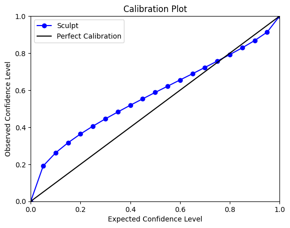
The calibration plot shows the relationship between the expected confidence level (x-axis) and the observed confidence level (y-axis). The blue line with markers represents the actual calibration of the Sculpt wrapped model. The blue calibration curve closely follows the black identity line, indicating that the model’s predicted uncertainties generally align well with the observed outcomes. This suggests that the model’s uncertainty estimates are fairly reliable.

Finally, we compute the expected calibration error. The Expected Calibration Error (ECE) is a metric used to quantify the difference between predicted probabilities and actual outcomes.

from themis_utils.calibration.calibration_metrics import expected_calibration_error

print('ECE:', expected_calibration_error(exp_conf, obs_conf))

ECE: 0.07947885422479538

The ECE value above shows the precentage of discrepancy between the predicted confidence levels and the observed confidence levels.