Use Case: Improve Sentiment Analysis with Mamba
Mamba was proposed in the paper Mamba: Linear-Time Sequence Modeling with Selective State Spaces. Mamba is a new state space model architecture concerned with sequence modeling. It was developed to address some limitations of transformer models, especially in processing long sequences, and has been showing promising performance.
You can find its official implementation and model checkpoints in its repository. In this tutorial, we will build the model from scratch in tensorflow, and demonstrate how to wrap with Sample wrapper.
Overview of Mamba
Transformers have seen recent popularity with the rise of Large Language Models (LLMs) like LLaMa-2, GPT-4, Claude, Gemini, etc., but it suffers from the problem of context window. The issue with transformers lies in it’s core, the multi head-attention mechanism. The main issue with multi-head attention sprouts from the fact that for input sequence length n, the time complexity and space complexity scales by O(n²). This limits the length of the context window of an LLM. Because, to increase it by 10x, we need to scale the hardware requirement (most notably GPU VRAM) by 100x. Mamba, on the other hand, scales by O(n)!, i.e., Linearly.
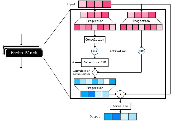
The Mamba architecture, after reading the paper and analysis of the code, can be broken into a few key components which are connected as:
Wrapping Mamba with Capsa-Tensorflow
Step 1: Imports
import tensorflow_datasets as tfds
import tensorflow as tf
from tensorflow import keras
from keras import layers, Model

from dataclasses import dataclass
from einops import rearrange, repeat
from typing import Union

from transformers import AutoTokenizer

import datasets
import math
import numpy as np

import capsa_tf #import our wrappers
import pickle
import matplotlib.pyplot as plt
Step 2: Create ModelArgs dataclass and load tokenizer
To make the modeling argument processing easier, let’s create a simple ModelArgs dataclass as a config class. This allows us to just pass the dataclass variable in the arguments when we are initializing the model.
@dataclass
class ModelArgs:
    model_input_dims: int = 64
    model_states: int = 64
    projection_expand_factor: int = 2
    conv_kernel_size: int = 4
    delta_t_min: float = 0.001
    delta_t_max: float = 0.1
    delta_t_scale: float = 0.1
    delta_t_init_floor: float = 1e-4
    conv_use_bias: bool = True
    dense_use_bias: bool = False
    layer_id: int = -1
    seq_length: int = 128
    num_layers: int = 5
    dropout_rate: float = 0.2
    use_lm_head: float = False
    num_classes: int = None
    vocab_size: int = None
    final_activation = None
    loss:Union[str, keras.losses.Loss] = None
    optimizer: Union[str, keras.optimizers.Optimizer] = keras.optimizers.AdamW()
    metrics = ['accuracy']

    def __post_init__(self):
        self.model_internal_dim: int = int(self.projection_expand_factor * self.model_input_dims)

        self.delta_t_rank = math.ceil(self.model_input_dims/16)
        if self.layer_id == -1:
            self.layer_id = np.round(np.random.randint(0, 1000), 4)

        if self.vocab_size == None:
            raise ValueError("vocab size cannot be none")

        if self.use_lm_head:
            self.num_classes=self.vocab_size
        else:
            if self.num_classes == None:
                raise ValueError(f'num classes cannot be {self.num_classes}')

            if self.num_classes == 1:
                self.final_activation = 'sigmoid'
            else:
                self.final_activation = 'softmax'

        if self.loss == None:
            raise ValueError(f"loss cannot be {self.loss}")

tokenizer = AutoTokenizer.from_pretrained("bert-base-uncased")
vocab_size = tokenizer.vocab_size
Step 3: Implement the parallel associative scan and Mamaba block
def selective_scan(u, delta, A, B, C, D):
    # first step of A_bar = exp(ΔA), i.e., ΔA
    dA = tf.einsum('bld,dn->bldn', delta, A)
    dB_u = tf.einsum('bld,bld,bln->bldn', delta, u, B)

    dA_cumsum = tf.pad(
        dA[:, 1:], [[0, 0], [1, 1], [0, 0], [0, 0]])[:, 1:, :, :]

    dA_cumsum = tf.reverse(dA_cumsum, axis=[1])  # Flip along axis 1

    # Cumulative sum along all the input tokens, parallel prefix sum,
    # calculates dA for all the input tokens parallely
    dA_cumsum = tf.math.cumsum(dA_cumsum, axis=1)

    # second step of A_bar = exp(ΔA), i.e., exp(ΔA)
    dA_cumsum = tf.exp(dA_cumsum)
    dA_cumsum = tf.reverse(dA_cumsum, axis=[1])  # Flip back along axis 1

    x = dB_u * dA_cumsum
    # 1e-12 to avoid division by 0
    x = tf.math.cumsum(x, axis=1)/(dA_cumsum + 1e-12)

    y = tf.einsum('bldn,bln->bld', x, C)

    return y + u * D

class MambaBlock(layers.Layer):
    def __init__(self, modelargs: ModelArgs, *args, **kwargs):
        super().__init__(*args, **kwargs)
        self.args = modelargs
        args = modelargs
        self.layer_id = modelargs.layer_id

        self.in_projection = layers.Dense(
            args.model_internal_dim * 2,
            input_shape=(args.model_input_dims,), use_bias=False)

        self.conv1d = layers.Conv1D(
            filters=args.model_internal_dim,
            use_bias=args.conv_use_bias,
            kernel_size=args.conv_kernel_size,
            groups=args.model_internal_dim,
            data_format='channels_first',
            padding='causal'
        )

        # this layer takes in current token 'x'
        # and outputs the input-specific Δ, B, C (according to S6)
        self.x_projection = layers.Dense(args.delta_t_rank + args.model_states * 2, use_bias=False)

        # this layer projects Δ from delta_t_rank to the mamba internal
        # dimension
        self.delta_t_projection = layers.Dense(args.model_internal_dim,
                                               input_shape=(args.delta_t_rank,), use_bias=True)

        self.A = repeat(
                tf.range(1, args.model_states+1, dtype=tf.float32),
                'n -> d n', d=args.model_internal_dim)

        self.A_log = tf.Variable(
                tf.math.log(self.A),
                trainable=True, dtype=tf.float32,
                name=f"SSM_A_log_{args.layer_id}")

        self.D = tf.Variable(
                np.ones(args.model_internal_dim),
                trainable=True, dtype=tf.float32,
                name=f"SSM_D_{args.layer_id}")

        self.out_projection = layers.Dense(
                args.model_input_dims,
                input_shape=(args.model_internal_dim,),
                use_bias=args.dense_use_bias)

    def call(self, x):
        """Mamba block forward. This looks the same as Figure 3 in Section 3.4 in the Mamba pape.
        Official Implementation:
            class Mamba, https://github.com/state-spaces/mamba/blob/main/mamba_ssm/modules/mamba_simple.py#L119
            mamba_inner_ref(), https://github.com/state-spaces/mamba/blob/main/mamba_ssm/ops/selective_scan_interface.py#L311
        """

        (batch_size, seq_len, dimension) = x.shape

        x_and_res = self.in_projection(x) # shape = (batch, seq_len, 2 * model_internal_dimension)
        (x, res) = tf.split(x_and_res,
                            [self.args.model_internal_dim,
                             self.args.model_internal_dim], axis=-1)

        x = rearrange(x, 'b l d_in -> b d_in l')
        x = self.conv1d(x)[:, :, :seq_len]
        x = rearrange(x, 'b d_in l -> b l d_in')

        x = tf.nn.swish(x)
        y = self.ssm(x)
        y = y * tf.nn.swish(res)
        return self.out_projection(y)

    def ssm(self, x):
        """Runs the SSM. See:
            - Algorithm 2 in Section 3.2 in the Mamba paper
            - run_SSM(A, B, C, u) in The Annotated S4
            Official Implementation:
            mamba_inner_ref(), https://github.com/state-spaces/mamba/blob/main/mamba_ssm/ops/selective_scan_interface.py#L311
        """
        (d_in, n) = self.A_log.shape

        # Compute ∆ A B C D, the state space parameters.
        #     A, D are input independent (see Mamba paper [1] Section 3.5.2 "Interpretation of A" for why A isn't selective)
        #     ∆, B, C are input-dependent (this is a key difference between Mamba and the linear time invariant S4,
        #                                  and is why Mamba is called **selective** state spaces)

        A = -tf.exp(tf.cast(self.A_log, tf.float32)) # shape -> (d_in, n)
        D = tf.cast(self.D, tf.float32)

        x_dbl = self.x_projection(x) # shape -> (batch, seq_len, delta_t_rank + 2*n)

        (delta, B, C) = tf.split(
                x_dbl,
                num_or_size_splits=[self.args.delta_t_rank, n, n],
                axis=-1) # delta.shape -> (batch, seq_len) & B, C shape -> (batch, seq_len, n)

        delta = tf.nn.softplus(self.delta_t_projection(delta)) # shape -> (batch, seq_len, model_input_dim)

        return selective_scan(x, delta, A, B, C, D)

class ResidualBlock(layers.Layer):
    def __init__(self, modelargs: ModelArgs, *args, **kwargs):
        super().__init__(*args, **kwargs)
        self.args = modelargs
        self.mixer = MambaBlock(modelargs)
        self.norm = layers.LayerNormalization(epsilon=1e-5)

    def call(self, x):
        """
        Official Implementation:
            Block.forward(), https://github.com/state-spaces/mamba/blob/main/mamba_ssm/modules/mamba_simple.py#L297

            Note: the official repo chains residual blocks that look like
                [Add -> Norm -> Mamba] -> [Add -> Norm -> Mamba] -> [Add -> Norm -> Mamba] -> ...
            where the first Add is a no-op. This is purely for performance reasons as this
            allows them to fuse the Add->Norm.

            We instead implement our blocks as the more familiar, simpler, and numerically equivalent
                [Norm -> Mamba -> Add] -> [Norm -> Mamba -> Add] -> [Norm -> Mamba -> Add] -> ....

        """
        return self.mixer(self.norm(x)) + x

def init_model(args: ModelArgs):
    input_layer = layers.Input(shape=(args.seq_length,), name='input_ids')
    x = layers.Embedding(args.vocab_size, args.model_input_dims, input_length=args.seq_length)(input_layer)

    for i in range(args.num_layers):
        x = ResidualBlock(args, name=f"Residual_{i}")(x)
        x = layers.Dropout(args.dropout_rate)(x)

    x = layers.LayerNormalization(epsilon=1e-5)(x)

    if not args.use_lm_head: # use flatten only if we are using the model as an LM
        x = layers.Flatten()(x)
    x = layers.Dense(1024, activation=tf.nn.gelu)(x)
    output_layer = layers.Dense(args.num_classes, activation=args.final_activation)(x)

    model = Model(inputs=input_layer, outputs=output_layer, name='Mamba_ka_Mamba',)
    model.compile(
        loss=args.loss,
        optimizer=args.optimizer,
        metrics=args.metrics,
    )

    return model
Step 4: Load data and initialize model
For this example, we will use the Mamba block to create a simple classification model. Let’s load the IMDB reviews dataset for a simple sentiment classifier.
dataset = load_dataset("ajaykarthick/imdb-movie-reviews")
args = ModelArgs(
model_input_dims=128,
model_states=32,
num_layers=12,
dropout_rate=0.2,
vocab_size=vocab_size,
num_classes=1,
loss='binary_crossentropy',
)
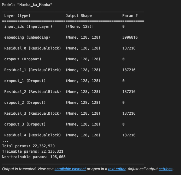
model = init_model(args)
model.summary()
We should see the output:
Step 5: Pre-tokenize data
train_labels, test_labels = [], []
train_ids = np.zeros((len(dataset['train']), args.seq_length))
test_ids = np.zeros((len(dataset['test']), args.seq_length))

for i, item in enumerate(tqdm(dataset['train'])):
    text = item['review']
    train_ids[i, :] = tokenizer.encode_plus(
            text,
            max_length=args.seq_length,
            padding='max_length',
            return_tensors='np')['input_ids'][0][:args.seq_length]

    train_labels.append(item['label'])

for i, item in enumerate(tqdm(dataset['test'])):
    text = item['review']
    test_ids[i, :] = tokenizer.encode_plus(
            text,
            max_length=args.seq_length,
            padding='max_length',
            return_tensors='np')['input_ids'][0][:args.seq_length]

    test_labels.append(item['label'])

del dataset # delete the original dataset to save some memory

BATCH_SIZE = 32
train_dataset = tf.data.Dataset.from_tensor_slices((train_ids, train_labels)).batch(BATCH_SIZE).shuffle(1000)
test_dataset = tf.data.Dataset.from_tensor_slices((test_ids, test_labels)).batch(BATCH_SIZE).shuffle(1000)
Step 6: Train model
def train_step(x,y):
    with tf.GradientTape() as tape:
        y_pred = wrapped_model(x, return_risk=False)#,tile_and_reduce=False)
        loss = model.compiled_loss(y, y_pred, regularization_losses=model.losses)

    capsa_vars, user_vars = wrapped_model.trainable_variables
    # For convenience, unpack these into a single flat list
    trainable_vars = [*capsa_vars, *user_vars]

    # Compute gradient of loss wrt all trainable_variables of the wrapped_model
    gradients = tape.gradient(loss, trainable_vars)
    # Update wrapped_model's trainable_variables with the computed gradient
    model.optimizer.apply_gradients(zip(gradients, trainable_vars))

    return loss


@capsa_tf.sample.Wrapper(inline=True)
def wrapped_model(*args, **kwargs):
    return model(*args, **kwargs)

base_model_path = "./training_checkpoints/cp_risk_sample_new-{epoch:04d}.ckpt"
wrapper_checkpoint_path = "./training_checkpoints/cp_risk_sample_new-{epoch:04d}.pkl"

#----------------------Training --------------------

training = True

if training:
  # Keep results for plotting
  train_loss_results = []
  train_accuracy_results = []

  num_epochs = 10

  best_val_loss = float('inf')

  for epoch in range(num_epochs):
    epoch_loss_avg = tf.keras.metrics.Mean()

    # Training loop - using batches of 32
    for x, y in train_dataset:
      loss_value=train_step(x,y)
      epoch_loss_avg.update_state(loss_value)
    # End epoch
    train_loss_results.append(epoch_loss_avg.result())

    val_loss_avg = tf.keras.metrics.Mean()
    for val_x, val_y in test_dataset:
        val_pred = wrapped_model(val_x, training=False)
        val_loss = model.compiled_loss(val_y, val_pred, regularization_losses=model.losses)
        val_loss_avg.update_state(val_loss)


    print("Epoch {:03d}: Train Loss: {:.3f}, Validation Loss: {:.3f}".format(epoch, epoch_loss_avg.result(), val_loss))

    # Save the model weights only if the validation loss has improved
    if val_loss < best_val_loss:
          best_val_loss = val_loss
          model.save_weights(base_model_path.format(epoch=epoch))
          PATH = wrapper_checkpoint_path.format(epoch=epoch)
          with open(PATH, "wb") as f:
            pickle.dump(wrapped_model.trainable_variables, f)
          print(f"Checkpoint saved at epoch {epoch} with validation loss {val_loss:.3f}")

else:
  latest = tf.train.latest_checkpoint('training_checkpoints')
  if latest:
      model.load_weights(latest)
      print(f"Loaded weights from {latest}")
  ckpt = tf.train.latest_checkpoint('training_checkpoints')
  out_pkl_iteration = ckpt.split('.ckpt')[0].split('/')[-1]
  out_pkl = 'training_checkpoints/'+out_pkl_iteration+'.pkl'
  with open(out_pkl, "rb") as f:
    restored_capsa_vars, restored_user_vars = pickle.load(f)
  wrapped_model.set_capsa_variables(restored_capsa_vars)
  print(f"Loaded weights for wrapped model from {out_pkl}")
Step 7: Visualize result
y_ls,flattened_pred_ls,flattened_risk_ls = [],[],[]
for test_x, test_y in test_dataset:
output=wrapped_model(test_x,training=False,return_risk=True)
y_ls.extend(test_y.numpy().flatten())
flattened_pred = output[0].numpy().flatten()
flattened_pred_ls.extend(flattened_pred)
flattened_risk = output[1].numpy().flatten()
flattened_risk_ls.extend(flattened_risk)
converted_pred_ls = (np.array(flattened_pred_ls) > 0.5).astype(np.int32)
# Convert lists to NumPy arrays
y_ls = np.array(y_ls)
flattened_pred_ls = np.array(flattened_pred_ls)
flattened_risk_ls = np.array(flattened_risk_ls)
converted_pred_ls = (flattened_pred_ls > 0.5).astype(np.int32)
# Compute accuracy
def compute_accuracy(y_true, y_pred):
return np.mean(y_true == y_pred)
# Sort by risk
sorted_indices = np.argsort(flattened_risk_ls)
sorted_y_ls = y_ls[sorted_indices]
sorted_converted_pred_ls = converted_pred_ls[sorted_indices]
sorted_risks = flattened_risk_ls[sorted_indices]
# Compute accuracy after removing top high-risk cases
def compute_accuracy_with_risk_threshold(y_true, y_pred, risks, threshold):
cutoff_index = int(len(risks) * (1 - threshold))
filtered_y_true = y_true[:cutoff_index]
filtered_y_pred = y_pred[:cutoff_index]
return compute_accuracy(filtered_y_true, filtered_y_pred)
# Define risk thresholds
risk_thresholds = np.linspace(0, 0.5, 11) # 0% to 50% in steps of 5%
accuracies = []
for threshold in risk_thresholds:
accuracy = compute_accuracy_with_risk_threshold(
sorted_y_ls, sorted_converted_pred_ls, sorted_risks, threshold
)
accuracies.append(accuracy)
print(f'Accuracy with top {threshold * 100:.0f}% high-risk cases removed: {accuracy:.4f}')
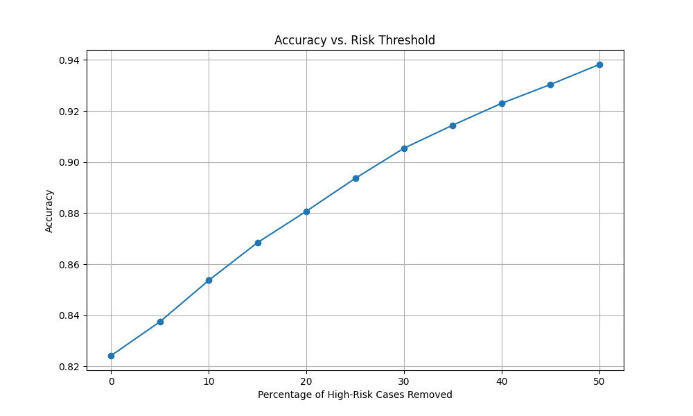
# Plot accuracy vs. risk threshold
plt.figure(figsize=(10, 6))
plt.plot(risk_thresholds * 100, accuracies, marker='o', linestyle='-')
plt.xlabel('Percentage of High-Risk Cases Removed')
plt.ylabel('Accuracy')
plt.title('Accuracy vs. Risk Threshold')
plt.grid(True)
plt.savefig('mamba_result.png')
plt.show()
We observe that the accuracy improves as we eliminate a greater number of high-risk cases.