Vote Wrapper: Generating MNIST Digits with VAE

In this tutorial we show how to wrap a VAE model and train it on MNIST dataset. Here we are using a Vote wrapper.

Step 1: Initial Setup

This step is universal and dependant to your specific model and dataset you are using. In this tutorial we are covering the steps needed to create a VAE model and load MNIST dataset.

import torch
import torch.nn as nn
import torch.nn.functional as F
import torch.utils
import torch.distributions
import torchvision
import numpy as np
import matplotlib.pyplot as plt
import tqdm

Note: Edit the line below to match your GPU information

device = "cuda:0" if torch.cuda.is_available() else "cpu"

Creating the Decoder module.

class Decoder(nn.Module):
    def __init__(self, latent_dims):
        super(Decoder, self).__init__()
        self.lin = nn.Linear(latent_dims, 32 * 7 * 7)
        self.decoder = nn.Sequential(
            nn.ReLU(),
            nn.ConvTranspose2d(32, 16, kernel_size=4, stride=2, padding=1),
            nn.ReLU(),
            nn.ConvTranspose2d(16, 1, kernel_size=4, stride=2, padding=1),
            nn.Sigmoid(),
        )

    def forward(self, z):
        z = self.lin(z)
        z = torch.reshape(z, (z.shape[0], 32, 7, 7))
        return self.decoder(z)

Creating the Encoder module.

class VariationalEncoder(nn.Module):
    def __init__(self, latent_dims):
        super(VariationalEncoder, self).__init__()
        self.encoder = nn.Sequential(
            nn.Conv2d(1, 16, kernel_size=3, stride=2, padding=1),
            nn.ReLU(),
            nn.Conv2d(16, 32, kernel_size=3, stride=2, padding=1),
            nn.ReLU(),
            nn.Flatten(),
        )
        self.fc_mu = nn.Linear(32 * 7 * 7, latent_dims)
        self.fc_sigma = nn.Linear(32 * 7 * 7, latent_dims)

        self.N = torch.distributions.Normal(0, 1)
        self.N.loc = self.N.loc.cuda(device)  # hack to get sampling on the GPU
        self.N.scale = self.N.scale.cuda(device)
        self.kl = 0

    def forward(self, x):
        x = self.encoder(x)
        mu = self.fc_mu(x)
        sigma = torch.exp(self.fc_sigma(x))
        z = mu + sigma * self.N.sample(mu.shape)
        self.kl = (sigma**2 + mu**2 - torch.log(sigma) - 1 / 2).sum()
        return z

Creating a VAE module

class VariationalAutoencoder(nn.Module):
    def __init__(self, latent_dims):
        super(VariationalAutoencoder, self).__init__()
        self.encoder = VariationalEncoder(latent_dims)
        self.decoder = Decoder(latent_dims)

    def forward(self, x):
        z = self.encoder(x)
        return self.decoder(z)

Loading the MNIST dataset

data = torch.utils.data.DataLoader(
    torchvision.datasets.MNIST(
        ".", transform=torchvision.transforms.ToTensor(), download=True
    ),
    batch_size=128,
    shuffle=True,
    drop_last=True,
)

The latent space dimension is set to 2 for easier visualization.

vae = VariationalAutoencoder(2).to(device)  # GPU

Step 2: Wrapping the model

In order to wrap your model with any wrapper you need to pass in the model along with a sample input to your model.

# Wrap the model
from capsa_torch import vote

x, y = next(iter(data))
x = x.cuda(device)
vae.decoder = vote.Wrapper(n_voters=2)(vae.decoder)

Note

Most wrappers require re-training or finetuning. Vote is one of the wrappers that requires re-training or finetuning and will not provide useful outputs otherwise. Read the wrapper documentations in order to pick the one that is suitable for your usecase.

Step 3: Training

Note

Add the tile_and_reduce=False flag for the Vote wrapper

opt = torch.optim.Adam(vae.parameters())
for epoch in range(20):
    for x, y in data:
        x = x.to(device)
        opt.zero_grad()
        z = vae.encoder(x)
        # NOTE: add the tile_and_reduce = False flag for the Vote Wrapper
        x_hat = vae.decoder(z, tile_and_reduce=False, return_risk=False)
        loss = ((x - x_hat) ** 2).sum() + vae.encoder.kl
        loss.backward()
        opt.step()

Step 4: Testing & Evaluation

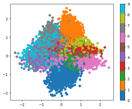
Once you have trained your wrapped model, you will get a risk value for every output to your model if return_risk = True. Before showing the risk predicted by the wrapper, you can visualize the outputs of the VAE in its first two dimensions, different colors indicate different labels. This gives a sense of what the distribution of reconstructed images looks like.

def plot_latent(autoencoder, data, num_batches=100):
    for i, (x, y) in enumerate(data):
        z = autoencoder.encoder(x.to(device))
        z = z.to('cpu').detach().numpy()
        plt.scatter(z[:, 0], z[:, 1], c=y, cmap='tab10')
        if i > num_batches:
            plt.colorbar()
            break
plot_latent(vae, data)

Then, you can plot the reconstructed images together with the risk estimated from Vote wrapper. The x and y axies in the plots are the two latent variables.

def normalize(arr):
    return (arr - np.min(arr))/(np.max(arr) - np.min(arr))


def plot_reconstructed(vae, r0=(-1, 1), r1=(-1, 1), n=12):
    w = 28
    img = np.zeros((n*w, n*w))
    risks = np.zeros((n*w, n*w))
    for i, y in enumerate(np.linspace(*r1, n)):
        for j, x in enumerate(np.linspace(*r0, n)):
            z = torch.Tensor([[x, y]]).to(device)
            x_hat, r = vae.decoder(z.repeat(64, 1), return_risk = True)
            x_hat = x_hat[0].reshape(28, 28).to('cpu').detach().numpy()
            r = r[0].reshape(28, 28).to('cpu').detach().numpy()
            img[(n-1-i)*w:(n-1-i+1)*w, j*w:(j+1)*w] = normalize(x_hat)
            risks[(n-1-i)*w:(n-1-i+1)*w, j*w:(j+1)*w] = normalize(r)
            
    fig = plt.figure()
    ax1 = fig.add_subplot(1,2,1)
    ax1.imshow(img, extent=[*r0, *r1])
    ax1.set_title("Reconstructed images")
    ax2 = fig.add_subplot(1,2,2)
    ax2.imshow(risks, extent=[*r0, *r1])
    ax2.set_title("Pixelwise uncertainty for\nthe reconstructed images")
    
    
plot_reconstructed(vae)

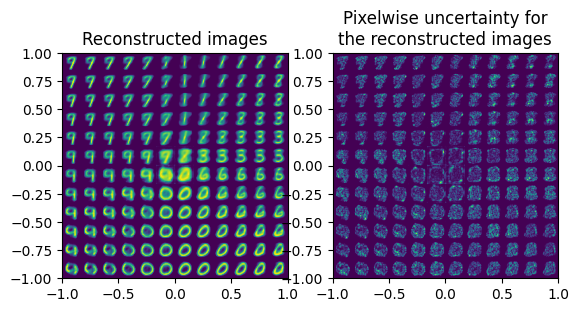
In the uncertainty results we can see, the high uncertainty mostly appears at the edges of digital number.