Neo Wrapper: Two Moons Classification

In this tutorial, we show how to wrap a simple MLP with Neo wrapper, and visualize the vacuity loss.

The “Two Moons” dataset is a popular synthetic dataset used in machine learning for visualizing clustering and classification algorithms. It consists of two interleaving half circles, often referred to as “moons.”

Step 1: Initial Setup

Import Dependencies

import torch
from torch import nn
from sklearn import datasets
import matplotlib.pyplot as plt
import numpy as np
import itertools
import tqdm
import os
device = torch.device("cuda:0")
torch.set_default_device(device)

Initialize Model

We define a simple linear model as the base model.

class BaseModel(torch.nn.Module):
    def __init__(self) -> None:
        super().__init__()

        self.linear0 = nn.Linear(2, 32)
        self.linear1 = nn.Linear(32, 32)
        self.linear2 = nn.Linear(32, 32)

        self.class_predictor = nn.Sequential(
            nn.Linear(32, 32), nn.ReLU(), nn.Linear(32, 2)
        )

    def forward(self, x):
        x = self.linear0(x)
        x = self.linear1(torch.relu(x))
        x = self.linear2(torch.relu(x))
        x = self.class_predictor(torch.relu(x))
        return x
model = BaseModel().to(device)

Create Dataset

# create your dataset
x, y = datasets.make_moons(n_samples=200, noise=0.1)
x = x.astype(float)
x = torch.from_numpy(x).to(torch.float32).to(device)
y = torch.from_numpy(y).to(device)
# create the grid
def get_grid():
    x = np.linspace(-2.5, 3.5, 200)
    y = np.linspace(-2.0, 2.5, 200)
    return np.array(list(itertools.product(x, y)))
mesh_grid = get_grid()

Train Base Model

Here we define a trainning function that can accomodate both regular (“unwrapped”) and Capsa-wrapped models. Unwrapped models are trained on the classification task, while the corresponding wrapped model will be trained to minimize the vacuity loss. This two-stage training process is required by the Neo wrapper.

def train_model(
    x: torch.Tensor, y: torch.Tensor, model, lr: float, steps: int, wrapped: bool):
    opt = torch.optim.Adam(model.parameters(), lr)
    cls_loss_fn = torch.nn.BCEWithLogitsLoss()

    loss_history = []
    prog_bar = tqdm.tqdm(range(steps), total=steps)
    for _ in prog_bar:
        if wrapped:
            logits, risk = model(x, return_risk=True)
            capsa_loss = risk.mean()
            loss = 0.01 * capsa_loss
        else:
            logits = model(x)
            cls_loss = cls_loss_fn(
                logits, torch.nn.functional.one_hot(y, 2).to(torch.float32)
            )
            loss = cls_loss

        opt.zero_grad()
        loss.backward()
        opt.step()

        loss_history.append(loss.item())
        prog_bar.set_postfix(loss=loss.item())

    return loss_history
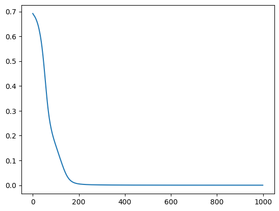
train_loss = train_model(x, y, model, lr=0.001, steps=1000, wrapped=False)
plt.plot(list(range(1000)), train_loss)
plt.show()

100%|██████████| 1000/1000 [00:03<00:00, 314.13it/s, loss=2.56e-5]

Step 2: Model Wrapping

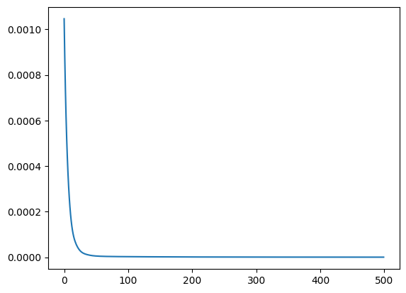
Here we use the Neo wrapper, which measures vacuitic uncertainty. The model wrapped with Neo Wrapper needs to be trained twice, first on the original classification task without considering the risk, which is done in the earlier step, then we train the wrapped model with the returned risk which is vacuity loss as the training loss.

from capsa_torch import neo

wrapper=neo.Wrapper(num_attachment_points=2,layers_spec=(4,4))

wrapped_model=wrapper(model)
wrapped_model=wrapped_model.to(device)

Training the Wrapped Model

Before beginning training, pass a sample of input data through the model (e.g., model(x)) to finalize the wrapping process. Below we use the evaluate_model function to do this, this step is necessary for any Neo wrapper trainning.

def evaluate_model(x: torch.Tensor, model):
    model.eval()
    with torch.no_grad():
        logits, risk = model(x, return_risk=True)
# pass a sample of input to finalize the wrapping
evaluate_model(x, wrapped_model)
# Train the model
STEPS = 500
LR = 0.001
train_loss = train_model(x, y, wrapped_model, lr=LR, steps=STEPS, wrapped=True)
plt.plot(list(range(STEPS)), train_loss)
plt.show()

100%|██████████| 500/500 [00:02<00:00, 202.52it/s, loss=2.18e-5] 

Step 3: Plot Vacuitic Uncertainty

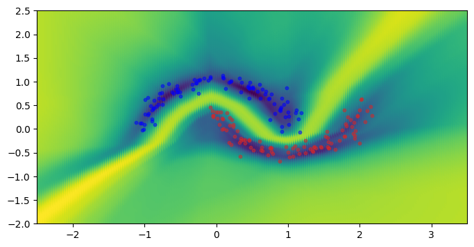
Vacuity uncertainty arises from a lack of evidence. A higher value indicates that the data point is less likely to have been drawn from the same distribution as the dataset. The Neo wrapper outputs a loss reflecting vacuity uncertainty, but this loss is unnormalized.

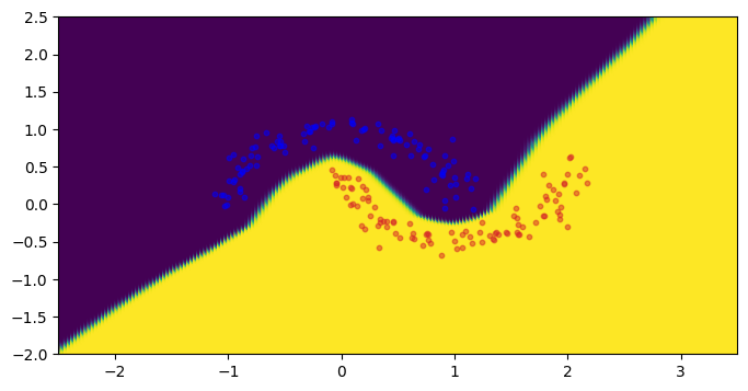
The first figure below shows the classification results, and the second figure is the corresponding vacuity loss.

def plot_mve_classification(output, mesh_grid, x_test, y_test):
    plt.figure(figsize=(8, 4))
    plt.xlim(min(mesh_grid[:, 0]), max(mesh_grid[:, 0]))
    plt.ylim(min(mesh_grid[:, 1]), max(mesh_grid[:, 1]))
    i = y_test == 0
    plt.scatter(x_test[i, 0], x_test[i, 1], s=10, alpha=0.5, c="b", zorder=-1)
    plt.scatter(
        x_test[~i, 0],
        x_test[~i, 1],
        s=10,
        alpha=0.5,
        c="#d62728",
        zorder=-1,
    )

    output = output.detach().cpu().numpy()
    plt.scatter(mesh_grid[:, 0], mesh_grid[:, 1], c=output, zorder=-2)
    
output = model(torch.from_numpy(mesh_grid).to(torch.float32).to(device))

plot_mve_classification(
        torch.softmax(output, -1)[:, 1], mesh_grid, x.cpu(), y.cpu()
    )
plt.show()

_, risk = wrapped_model(torch.from_numpy(mesh_grid).to(torch.float32).to(device), return_risk=True)
plot_mve_classification(torch.log(risk), mesh_grid, x.cpu(), y.cpu())
plt.show()

In areas where we have a higher density of data points, we see that the vacuity loss is low. This is consistent with our intuition.