Sculpt Wrapper: Regression
In this tutorial we show how to wrap a simple regression model with Capsa Sculpt wrapper in Tensorflow.
We will demonstrate how the Sculpt-wrapped model is able to provide valuable insights into the model and data, beyond what a typical deep neural network model is capable of.
Suppose we are given a training dataset consisting of observation pairs \((x_i,y_i)\) for \(i = 1, 2,\dots\) where the outputs \(y_i\) are modelled as
The variable \(\epsilon\) represents noise (or volatility) in the output \(y\), and measures deviation from the base model \(y = x + \sin(2x)\). This noise is heteroscedastic since its variance \(\sigma(x)^2\) varies with \(x\); specifically, we consider
This type of model and noise can approximate some real world applications. For example, financial markets tend to follow relatively cyclic patterns, punctuated by periods of high volatility (risk).
Step 1: Initial Setup
To begin, we’ll generate some training data from the model described above.
import tensorflow as tf
import math
import matplotlib.pyplot as plt
import numpy as np

tf.random.set_seed(1)
np.random.seed(1)
np.set_printoptions(threshold=10)


def fn(x):
    y = np.sin(2*x) + x
    high_risk_x = (x > 0) & (x < np.pi / 2)
    noise = np.random.normal(0, 1, x.shape) * high_risk_x + np.random.normal(0, 0.2, x.shape) * ~high_risk_x
    y += noise
    return y

x = np.linspace(-math.pi,math.pi,1000)[:, np.newaxis]
y = fn(x)

x = tf.convert_to_tensor(x, dtype=tf.float32)
y = tf.convert_to_tensor(y, dtype=tf.float32)
2025-09-30 18:51:11.915493: E external/local_xla/xla/stream_executor/cuda/cuda_fft.cc:479] Unable to register cuFFT factory: Attempting to register factory for plugin cuFFT when one has already been registered
2025-09-30 18:51:11.932442: E external/local_xla/xla/stream_executor/cuda/cuda_dnn.cc:10575] Unable to register cuDNN factory: Attempting to register factory for plugin cuDNN when one has already been registered
2025-09-30 18:51:11.932467: E external/local_xla/xla/stream_executor/cuda/cuda_blas.cc:1442] Unable to register cuBLAS factory: Attempting to register factory for plugin cuBLAS when one has already been registered
2025-09-30 18:51:11.944532: I tensorflow/core/platform/cpu_feature_guard.cc:210] This TensorFlow binary is optimized to use available CPU instructions in performance-critical operations.
To enable the following instructions: AVX2 FMA, in other operations, rebuild TensorFlow with the appropriate compiler flags.
2025-09-30 18:51:12.571018: W tensorflow/compiler/tf2tensorrt/utils/py_utils.cc:38] TF-TRT Warning: Could not find TensorRT
2025-09-30 18:51:13.547900: I external/local_xla/xla/stream_executor/cuda/cuda_executor.cc:998] successful NUMA node read from SysFS had negative value (-1), but there must be at least one NUMA node, so returning NUMA node zero. See more at https://github.com/torvalds/linux/blob/v6.0/Documentation/ABI/testing/sysfs-bus-pci#L344-L355
2025-09-30 18:51:13.550886: I external/local_xla/xla/stream_executor/cuda/cuda_executor.cc:998] successful NUMA node read from SysFS had negative value (-1), but there must be at least one NUMA node, so returning NUMA node zero. See more at https://github.com/torvalds/linux/blob/v6.0/Documentation/ABI/testing/sysfs-bus-pci#L344-L355
2025-09-30 18:51:13.553803: I external/local_xla/xla/stream_executor/cuda/cuda_executor.cc:998] successful NUMA node read from SysFS had negative value (-1), but there must be at least one NUMA node, so returning NUMA node zero. See more at https://github.com/torvalds/linux/blob/v6.0/Documentation/ABI/testing/sysfs-bus-pci#L344-L355
2025-09-30 18:51:13.558748: I external/local_xla/xla/stream_executor/cuda/cuda_executor.cc:998] successful NUMA node read from SysFS had negative value (-1), but there must be at least one NUMA node, so returning NUMA node zero. See more at https://github.com/torvalds/linux/blob/v6.0/Documentation/ABI/testing/sysfs-bus-pci#L344-L355
2025-09-30 18:51:13.619975: W tensorflow/core/common_runtime/gpu/gpu_device.cc:2251] Cannot dlopen some GPU libraries. Please make sure the missing libraries mentioned above are installed properly if you would like to use GPU. Follow the guide at https://www.tensorflow.org/install/gpu for how to download and setup the required libraries for your platform.
Skipping registering GPU devices...
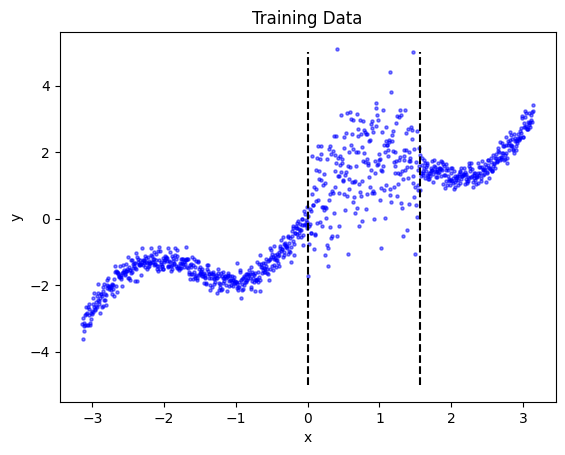
When plotting the data, we can see the dramatic change in the volatility (aleatoric risk) between \(x=0\) and \(x=\pi/2\).
plt.scatter(x, y, label='Ground truth data', s=5, c='blue',alpha=0.5)
plt.vlines([0,np.pi/2], -5, 5, linestyle='dashed', color='k')
plt.xlabel('x')
plt.ylabel('y')
plt.title('Training Data')
plt.show()
In this tutorial we will model the data using a simple sequential deep learning model consisting of 4 fully-connected layers.
initializer = tf.keras.initializers.GlorotNormal(seed=123)
W1 = tf.Variable(initializer(shape=(1, 64)))
W2 = tf.Variable(initializer(shape=(64, 64)))
W3 = tf.Variable(initializer(shape=(64, 64)))
W4 = tf.Variable(initializer(shape=(64, 1)))

initializer = tf.keras.initializers.Constant(0.05)
B1 = tf.Variable(initializer(shape=(64)))
B2 = tf.Variable(initializer(shape=(64)))
B3 = tf.Variable(initializer(shape=(64)))
B4 = tf.Variable(initializer(shape=(1)))

@tf.function
def model(x):
    x = tf.matmul(x, W1) + B1
    x = tf.nn.relu(x)
    x = tf.matmul(x, W2) + B2
    x = tf.nn.relu(x)
    x = tf.matmul(x, W3) + B3
    x = tf.nn.relu(x)
    x = tf.matmul(x, W4) + B4
    return x
Step 2: Wrapping the model
Wrapping the model is as simple as importing sculpt from the capsa_tf and wrapping the model with a sculpt.Wrapper object. This object requires a single argument, the distribution type with which to model the aleatoric risk. In this case, we use the normal (Gaussian) distribution, sculpt.Normal. The wrapper will produce better risk estimates if the selected distribution is close to the actual noise distribution, but the normal distribution is a good approximation in many cases.
from capsa_tf import sculpt

# Wrap model with sculpt wrapper
dist = sculpt.Normal
wrapped_model = sculpt.Wrapper(dist, n_layers=2)(model)
/tmp/ipykernel_3074791/742637034.py:1: CapsaWarning: Keras is not supported for tensorflow<2.17. (tensorflow version '2.16.2' is lower than the recommended minimum of '2.17.0'.)
  from capsa_tf import sculpt
When used normally, the wrapped model functions exactly the same way as the original model.
original_predictions = model(x)
wrapped_predictions = wrapped_model(x)
if tf.equal(tf.cast(tf.math.reduce_all(original_predictions == wrapped_predictions), tf.int32), 1):
    print('Wrapped model outputs match original model')
else:
    print('Wrapped model outputs DO NOT match original model')
Wrapped model outputs match original model
However, the wrapped model takes an optional keyword argument, return_risk, which outputs aleatoric risk when set to True, as seen below.
pred, risk = wrapped_model(x, return_risk=True)
if tf.equal(tf.cast(tf.math.reduce_all(original_predictions == pred), tf.int32), 1):
    print('Wrapped model outputs still match original model')
else:
    print('Wrapped model outputs DO NOT match original model')

print('Predictions:', tf.transpose(pred))  # transposed for prettier printing
print('Risk:', tf.transpose(risk))
Wrapped model outputs still match original model
Predictions: tf.Tensor([[0.15077986 0.15070577 0.15063186 ... 0.68953186 0.6905047  0.6914776 ]], shape=(1, 1000), dtype=float32)
Risk: tf.Tensor([[2.1531339 2.1536217 2.154109  ... 2.410312  2.4097762 2.4092405]], shape=(1, 1000), dtype=float32)
Step 3: Training
Most wrappers require re-training or finetuning in order to produce accurate risk estimates. Sculpt is one of these wrappers: it will not provide useful outputs unless the model is re-trained or finetuned. Furthermore, it requires a one-line modification to the original training procedure, which we demonstrate below.
Note
Read the wrapper documentations in order to pick the wrapper most suitable for your use case.
def train_step(x, y):
    with tf.GradientTape() as tape:
        y_hat, risk = wrapped_model(x, return_risk=True)

        ### NEW ###
        # Using the sculpt wrapper requires using a distribution-specific loss function, like this:
        loss = dist.loss_function(y, y_hat, risk)
        ### The rest of the code in this block is typical Tensorflow training code ###

        # The following line is optional:
        # loss += _YOUR_ORIGINAL_LOSS_FUNCTION

    trainable_vars = tape.watched_variables()
    gradients = tape.gradient(loss, trainable_vars)
    optimizer.apply_gradients(zip(gradients, trainable_vars))

    return loss

# train
optimizer = tf.optimizers.Adam(learning_rate=1e-4)
total_loss = []
n_epochs = 2500

for ep in range(n_epochs):
    loss = train_step(x, y)
    print(f'epoch: {ep+1}/{n_epochs}, mean loss: {loss}', end='\r')
    total_loss.append(loss)
epoch: 2500/2500, mean loss: -0.695630848407745465
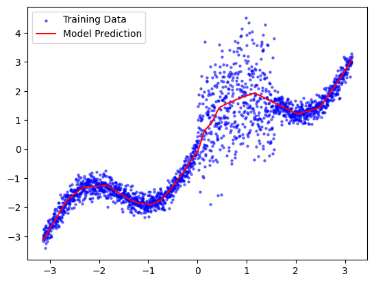
Now that we’ve trained the (wrapped) model, we can plot its predictions to verify that it learned a good approximation of the base function. We’ll use some new test data generated from the same model.
test_x = np.linspace(-math.pi,math.pi,2000)[:, np.newaxis]
test_y = fn(test_x)

test_x = tf.convert_to_tensor(test_x, dtype=tf.float32)
test_y = tf.convert_to_tensor(test_y, dtype=tf.float32)

test_predictions = wrapped_model(test_x)

plt.scatter(test_x, test_y, label='Training Data', s=5, c='blue',alpha=0.5)
plt.plot(test_x, test_predictions, label='Model Prediction', c='red')
_ = plt.legend(loc='best')
Step 4: Risk Evaluation
Finally, let’s take a look at the wrapped model’s risk estimates. Since we used the Sculpt wrapper, we expect that the risk will represent the aleatoric uncertainty (or “volatility”) in the outputs. More specifically, it represents the standard deviation of the output.
Since we are using a Normal distribution approximation, we expect that 95% of the output data should lie within 2 standard deviations of the predicted output. We visualize and test this below.
y_pred, risk = wrapped_model(test_x, return_risk = True)

# Convert to numpy for easier plotting
x_np, y_np, y_pred_np, risk_np = test_x.numpy(), test_y.numpy(), y_pred.numpy(), risk.numpy()
plt.fill_between(x_np.ravel(), y_pred_np.ravel()+2*risk_np.ravel(),y_pred_np.ravel()-2*risk_np.ravel(),color='orange',alpha=1, label='95% Confidence Interval')
plt.scatter(x_np, y_np, label='Ground truth data', s=5, c='blue',alpha=0.5)
plt.plot(x_np, y_pred_np, label='Prediction', c='red')
plt.legend(loc='best')

within_two_std = (np.abs(y_np - y_pred) < 2 * risk_np).sum()
perc_within_two_std = within_two_std / y_np.size
print(f'{perc_within_two_std*100:.1f}% of the data points are within two standard deviations')
93.8% of the data points are within two standard deviations
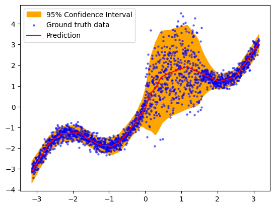
The results above suggest that the Sculpt wrapper accurately captures the distribution of the outputs. In fact, since we know the true volatility (risk) function, we can evaluate the predicted risk directly, as we do below, and see that the risk estimates are nearly perfect.
plt.plot(x_np, risk_np, label='Estimated Risk', c='green')
plt.plot([-np.pi, 0, 0, np.pi/2, np.pi/2, np.pi], [0.2,0.2,1,1,0.2,0.2], 'k--', label='Actual Risk')
plt.ylim([0,None])
plt.legend(loc='best')
_ = plt.title('Sculpt Wrapper Risk (Volatility) Estimate')
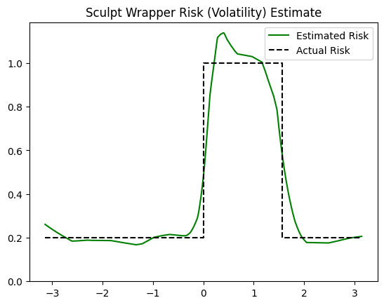
Note that slight deviation between the estimated and actual volatility estimates are expected due to the stochasticity of training, the limited training data, and the inability of the model to perfectly capture the instantaneous change (step function) in volatility. With a larger model and more training data, the estimates would improve even further.
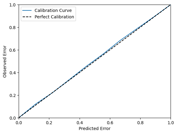
We can further evaluate the volatility estimates by plotting the regression calibration curve, which shows the actual percentage of points within an n’th percentile deviation from the mean. As expected, since the simulated data is normally distributed, the calibration is nearly perfect.
!pip install -q themis-utils[calib]

from themis_utils.calibration import regression_calibration_curve

exp_conf, obs_conf = regression_calibration_curve(test_y.numpy().flatten(), test_predictions.numpy().flatten(), risk.numpy().flatten(), num_samples=10)

plt.figure()
ax = plt.gca()
ax.plot(exp_conf, obs_conf, label='Calibration Curve')
ax.plot([0, 1], [0, 1], '--', color='black', label='Perfect Calibration')
plt.xlabel('Predicted Error')
plt.ylabel('Observed Error')
plt.xlim([0, 1])
plt.ylim([0, 1])
ax.legend()
plt.show()