Sculpt Wrapper: Regression

In this tutorial we show how to wrap a simple regression model with Capsa Sculpt Wrapper. The Sculpt wrapper predicts aleatoric uncertainty, which increases in regions where the relationship between inputs and outputs is noisy or ambiguous. This differs from epistemic uncertainty, which increases training data is sparse or absent (compare with the vote wrapper regression tutorial).

Step 1: Initial Setup

This step is universal and dependant to your specific model and dataset you are using.

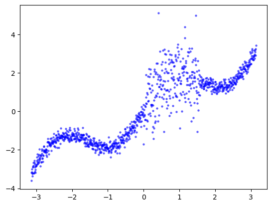
In this example our goal is to estimate a sinusoidal function. We generate synthetic data adding randomness to the function, where the randomness in one area is much larger than the rest, and predict it with a simple neural network.

import torch
import math
import tqdm
import numpy as np
import matplotlib.pyplot as plt

torch.manual_seed(1)
np.random.seed(1)

def fn(x):
    y = np.sin(2*x) + x
    high_risk_x = (x > 0) & (x < np.pi / 2)
    noise = np.random.normal(0, 1, x.shape) * high_risk_x + np.random.normal(0, 0.2, x.shape) * ~high_risk_x
    y += noise
    return y

x = np.linspace(-math.pi,math.pi,1000)[:, np.newaxis]
y = fn(x)

x = torch.Tensor(x)
y = torch.Tensor(y)

plt.scatter(x, y, label='Ground truth data', s=5, c='blue',alpha=0.5)
plt.show()

In this tutorial we are using a simple sequential model.

from torch import nn

def init_weights(m):
    if isinstance(m, nn.Linear):
        torch.nn.init.xavier_normal_(m.weight)
        if m.bias is not None:
            torch.nn.init.constant_(m.bias, 0.05)

model = nn.Sequential(nn.Linear(1, 64),
            nn.ReLU(),
            nn.Linear(64, 64),
            nn.ReLU(),
            nn.Linear(64, 64),
            nn.ReLU(),
            nn.Linear(64, 1))
model.apply(init_weights)

Sequential(
  (0): Linear(in_features=1, out_features=64, bias=True)
  (1): ReLU()
  (2): Linear(in_features=64, out_features=64, bias=True)
  (3): ReLU()
  (4): Linear(in_features=64, out_features=64, bias=True)
  (5): ReLU()
  (6): Linear(in_features=64, out_features=1, bias=True)
)

Step 2: Wrapping the model

In order to wrap your model with any wrapper you need to pass in the model along with a sample input to your model. The Sculpt wrapper can output a risk after wrapped, however, the risk is not useful before further training (even if the unwrapped model is already trained).

from capsa_torch import sculpt
#Wrap model with sculpt wrapper
dist = sculpt.Normal
wrapped_model = sculpt.Wrapper(dist, torch_compile=True, n_layers=2)(model)

with torch.no_grad():
    pred, risk = wrapped_model(x, return_risk=True)

learning_rate = 1e-4

opt = torch.optim.Adam(model.parameters(), lr = learning_rate)

Note

Most wrappers require re-training or finetuning. Sculpt is one of the wrappers that requires re-training or finetuning and will not provide useful outputs otherwise. Read the wrapper documentations in order to pick the one that is suitable for your usecase.

Step 3: Training

prog_bar = tqdm.trange(3000)
for t in prog_bar:
    #The model now returns 2 outputs (when return_risk=True)
    y_pred, risk = wrapped_model(x, return_risk = True)
    # Use the loss term for your distribution
    loss = dist.loss_function(y, y_pred, risk) - np.log(2 * torch.pi) / 2.

    opt.zero_grad()
    loss.backward()
    opt.step()
    prog_bar.set_postfix(loss = loss.item())

100%|██████████| 3000/3000 [00:13<00:00, 226.43it/s, loss=-0.642]  

with torch.no_grad():
    y_pred_train, risk_train = wrapped_model(x, return_risk = True)
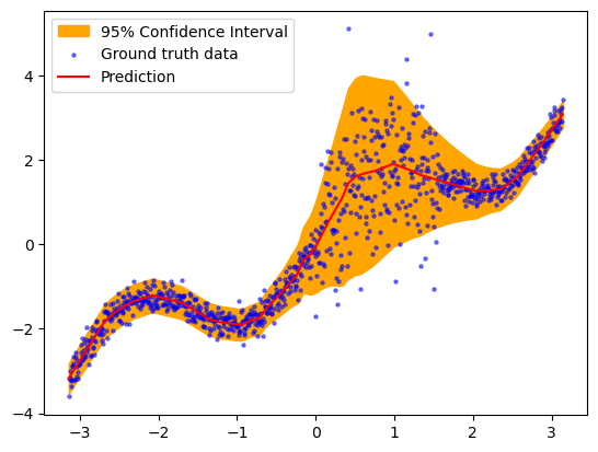
plt.fill_between(x.ravel(), y_pred_train.detach().ravel()+2*risk_train.ravel(),y_pred_train.detach().ravel()-2*risk_train.ravel(),color='orange',alpha=1, label='95% Confidence Interval')
plt.scatter(x, y, label='Ground truth data', s=5, c='blue',alpha=0.5)
plt.plot(x, y_pred_train.detach(), label='Prediction', c='red')
plt.legend(loc='best')

<matplotlib.legend.Legend at 0x7531161b7310>

Step 4: Testing & Evaluation

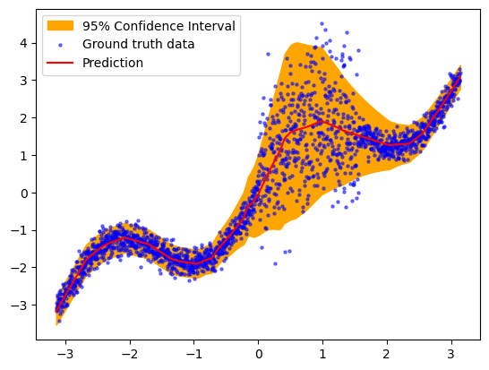
Once you have trained your wrapped model, you will get a risk value for every output to your model if return_risk = True. Here, you can visualize the predicted risk as the orange filling area in the plot.

#Generate testing data
x_test = torch.linspace(-math.pi, math.pi, 2000).unsqueeze(-1)
y_test = torch.Tensor(fn(x_test.numpy()))

with torch.no_grad():
    y_pred_test, risk_test = wrapped_model(x_test, return_risk = True)
plt.fill_between(x_test.ravel(), y_pred_test.detach().ravel()+2*risk_test.ravel(),y_pred_test.detach().ravel()-2*risk_test.ravel(),color='orange',alpha=1, label='95% Confidence Interval')
plt.scatter(x_test, y_test, label='Ground truth data', s=5, c='blue',alpha=0.5)
plt.plot(x_test, y_pred_test.detach(), label='Prediction', c='red')
plt.legend(loc='best')

<matplotlib.legend.Legend at 0x7530887ba4d0>

plt.plot(x_test, risk_test, label='Sculpt Wrapper Risk', c='green')
plt.plot([-np.pi, 0, 0, np.pi/2, np.pi/2, np.pi], [0.2,0.2,1,1,0.2,0.2], 'k--', label='Actual Risk')
plt.legend(loc='best')

<matplotlib.legend.Legend at 0x753088636d10>

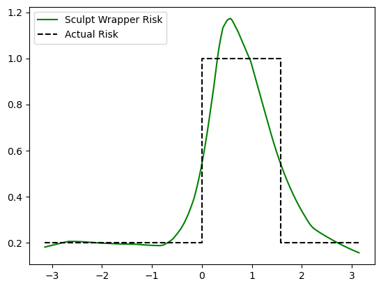
Note that slight deviation between the estimated and actual volatility estimates are expected due to the stochasticity of training, the limited training data, and the inability of the model to perfectly capture the instantaneous change (step function) in volatility. With a larger model and more training data, the estimates would improve even further.

We can further evaluate the volatility estimates by plotting the regression calibration curve, which shows the actual percentage of points within an n’th percentile deviation from the mean. As expected, since the simulated data is normally distributed, the calibration is nearly perfect.

!pip install -q themis-utils[calib]

from themis_utils.calibration import regression_calibration_curve

exp_conf, obs_conf = regression_calibration_curve(y_test.numpy().flatten(), y_pred_test.detach().numpy().flatten(), risk_test.numpy().flatten(), num_samples=10)

plt.figure()
ax = plt.gca()
ax.plot(exp_conf, obs_conf, label='Calibration Curve')
ax.plot([0, 1], [0, 1], '--', color='black', label='Perfect Calibration')
plt.xlabel('Predicted Error')
plt.ylabel('Observed Error')
plt.xlim([0, 1])
plt.ylim([0, 1])
ax.legend()
plt.show()