Use Case: Inspecting and Removing Bias from CelebA

In this tutorial, we show how to wrap a ResNet model with Neo wrapper, and based on the results we can analyze the bias in the dataset and model, then resample the dataset with a debiased scheme.

CelebFaces Attributes Dataset (CelebA) is a large-scale face attributes dataset with more than 200K celebrity images, each with 40 binary attribute annotations.

Step 1: Initial Setup

Download CelebA dataset and model weights

1. Download the dataset here. Unzip the data into folder “…/CelebA”

2. Download the weights here and place the .pth file in the folder where this notebook is located

3. The weights used for the base model were trained from the github repo: https://github.com/blingenf/celeba-baselines, using the dataset class for CelebA, which is celeba.py.

You should setup your dataset structure as described here, using the aligned images.

Import Dependencies

import numpy as np
import torch
import torch.nn as nn
import torch.optim as optim
import torch.nn.functional as F
from torch.utils.data import Dataset, DataLoader
from torchvision import models, datasets, transforms
import torchvision.transforms.functional as TF
from urllib.request import urlopen
from glob import glob
from celeba import CelebA
import sys
import time
import matplotlib.pyplot as plt
import matplotlib.cm as cm
from matplotlib.offsetbox import OffsetImage, AnnotationBbox
import matplotlib.gridspec as gridspec
import os
from sklearn.manifold import TSNE
CELEBA_DIR = "CelebA"

Define and initialize the model

The base model is ResNet18, we simply need to change the last layer from 1000 outputs to 40, then load the trained weights.

import warnings
warnings.filterwarnings("ignore")
class AttributeNN(nn.Module):
    """Base network for learning representations. Just a wrapper for
    ResNet18 which maps the last layer to 40 outputs instead of the
    1000 used for ImageNet classification.
    """
    def __init__(self, n_labels, pretrain=False):
        super().__init__()
        self.resnet = models.resnet18(pretrained=pretrain)
        self.fc_in_feats = self.resnet.fc.in_features

        self.resnet.fc = nn.Linear(self.fc_in_feats, n_labels, bias=True)
        self.n_labels = n_labels

    def forward(self, input):
        output = self.resnet(input)
        return output

saved_model_path = 'resnet18_multiplicative'
device='cuda'
saved_state_dict = torch.load(saved_model_path)
model = AttributeNN(40)
model = model.to(device)

# Load the updated state_dict into the model
model.load_state_dict(saved_state_dict)

<All keys matched successfully>

Step 2: Wrap with Capsa-Torch and Train Model

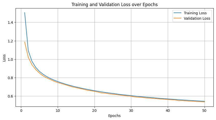
Here we use the Neo Wrapper which yields vacuity loss. The model wrapped with Neo Wrapper must be trained, here we provide the training code, and also the weights trained with the same setup for you to load.

from capsa_torch import neo

wrapper=neo.Wrapper()

wrapped_model=wrapper(model)
wrapped_model=wrapped_model.to(device)

Define Training Loop

def evaluate(network, dataloader):
    with torch.no_grad():
            for batch, _ in dataloader:
                batch = batch.to(device)
                output, risk = network(batch, return_risk=True)


def train(network, dataloader, dataloader_val, lr, epochs, device, model_name, patience=5, delta=0):
    """Simplified function for training the Wrapped_AttributeNN model with early stopping."""

    optimizer = optim.SGD(network.parameters(),
                          lr=lr, momentum=0.9, weight_decay=0.0001)

    training_losses = []
    validation_losses = []

    best_val_loss = float('inf')
    epochs_no_improve = 0 

    network.train()
    for epoch in range(epochs):
        start_time = time.time()
        avg_loss = 0
        for i, (batch, _) in enumerate(dataloader):
            batch = batch.to(device)

            optimizer.zero_grad()

            output, risk = network(batch, return_risk=True)

            # Compute the loss
            loss = risk.mean()

            loss.backward()
            optimizer.step()

            avg_loss += loss.item()

        avg_loss /= len(dataloader)
        training_losses.append(avg_loss)

        print(f"Epoch [{epoch + 1}/{epochs}], Training Loss: {avg_loss:.4f}, Time: {time.time() - start_time:.2f}s")
        sys.stdout.flush()

        #torch.save(network.state_dict(), f"{model_name}_epoch_{epoch + 1}.pth")

        network.eval()
        with torch.no_grad():
            avg_val_loss = 0
            for batch, _ in dataloader_val:
                batch = batch.to(device)

                output, risk = network(batch, return_risk=True)

                loss = risk.mean()
                avg_val_loss += loss.item()

            avg_val_loss /= len(dataloader_val)
            validation_losses.append(avg_val_loss)

        print(f"Epoch [{epoch + 1}/{epochs}], Validation Loss: {avg_val_loss:.4f}")
        sys.stdout.flush()

        # Early stopping logic
        if avg_val_loss < best_val_loss - delta:
            best_val_loss = avg_val_loss
            epochs_no_improve = 0 
            torch.save(network.state_dict(), f"{model_name}_best.pth")  # Save the best model
        else:
            epochs_no_improve += 1

        if epochs_no_improve >= patience:
            print(f"Early stopping at epoch {epoch + 1}. Best validation loss: {best_val_loss:.4f}")
            break

        network.train()

    # Plot training and validation losses
    plt.figure(figsize=(10, 5))
    plt.plot(range(1, epochs + 1), training_losses, label='Training Loss')
    plt.plot(range(1, epochs + 1), validation_losses, label='Validation Loss')
    plt.xlabel('Epochs')
    plt.ylabel('Loss')
    plt.title('Training and Validation Loss over Epochs')
    plt.legend()
    plt.grid(True)
    plt.show()

Load Data and Start Training

# Load your dataset
dataset = CelebA(CELEBA_DIR, fold='train', use_transforms=True, normalize=False)
dataloader = DataLoader(dataset, batch_size=32, shuffle=True, num_workers=4)

dataset_val = CelebA(CELEBA_DIR, fold='val', use_transforms=True, normalize=False)
dataloader_val = DataLoader(dataset_val, batch_size=32, shuffle=False, num_workers=4)

dataset_test = CelebA(CELEBA_DIR, fold='test', use_transforms=True, normalize=False)
dataloader_test = DataLoader(dataset_test, batch_size=1, shuffle=False, num_workers=4)
evaluate(wrapped_model, dataloader_val)
# Train the model
train(wrapped_model, dataloader, dataloader_val, lr=0.0001, epochs=50, device='cuda', model_name="Wrapped_AttributeNN")

Epoch [1/50], Training Loss: 0.5152, Time: 185.21s
Epoch [1/50], Validation Loss: 0.4035
Epoch [2/50], Training Loss: 0.3597, Time: 183.25s
Epoch [2/50], Validation Loss: 0.3234
Epoch [3/50], Training Loss: 0.3008, Time: 182.16s
Epoch [3/50], Validation Loss: 0.2783
Epoch [4/50], Training Loss: 0.2600, Time: 184.06s
Epoch [4/50], Validation Loss: 0.2415
Epoch [5/50], Training Loss: 0.2289, Time: 184.09s
Epoch [5/50], Validation Loss: 0.2153
Epoch [6/50], Training Loss: 0.2046, Time: 183.91s
Epoch [6/50], Validation Loss: 0.1940
Epoch [7/50], Training Loss: 0.1854, Time: 183.52s
Epoch [7/50], Validation Loss: 0.1765
Epoch [8/50], Training Loss: 0.1701, Time: 183.27s
Epoch [8/50], Validation Loss: 0.1640
Epoch [9/50], Training Loss: 0.1579, Time: 185.93s
Epoch [9/50], Validation Loss: 0.1524
Epoch [10/50], Training Loss: 0.1479, Time: 183.67s
Epoch [10/50], Validation Loss: 0.1433
Epoch [11/50], Training Loss: 0.1397, Time: 184.57s
Epoch [11/50], Validation Loss: 0.1369
Epoch [12/50], Training Loss: 0.1329, Time: 183.78s
Epoch [12/50], Validation Loss: 0.1305
Epoch [13/50], Training Loss: 0.1272, Time: 184.11s
Epoch [13/50], Validation Loss: 0.1244
Epoch [14/50], Training Loss: 0.1224, Time: 186.01s
Epoch [14/50], Validation Loss: 0.1201
Epoch [15/50], Training Loss: 0.1183, Time: 184.40s
Epoch [15/50], Validation Loss: 0.1167
Epoch [16/50], Training Loss: 0.1148, Time: 185.29s
Epoch [16/50], Validation Loss: 0.1129
Epoch [17/50], Training Loss: 0.1117, Time: 184.96s
Epoch [17/50], Validation Loss: 0.1104
Epoch [18/50], Training Loss: 0.1090, Time: 184.09s
Epoch [18/50], Validation Loss: 0.1078
Epoch [19/50], Training Loss: 0.1065, Time: 185.03s
Epoch [19/50], Validation Loss: 0.1053
Epoch [20/50], Training Loss: 0.1044, Time: 185.54s
Epoch [20/50], Validation Loss: 0.1034
Epoch [21/50], Training Loss: 0.1024, Time: 183.86s
Epoch [21/50], Validation Loss: 0.1014
Epoch [22/50], Training Loss: 0.1006, Time: 185.72s
Epoch [22/50], Validation Loss: 0.0996
Epoch [23/50], Training Loss: 0.0990, Time: 185.01s
Epoch [23/50], Validation Loss: 0.0981
Epoch [24/50], Training Loss: 0.0975, Time: 187.54s
Epoch [24/50], Validation Loss: 0.0969
Epoch [25/50], Training Loss: 0.0961, Time: 184.31s
Epoch [25/50], Validation Loss: 0.0957
Epoch [26/50], Training Loss: 0.0948, Time: 184.50s
Epoch [26/50], Validation Loss: 0.0943
Epoch [27/50], Training Loss: 0.0936, Time: 183.51s
Epoch [27/50], Validation Loss: 0.0930
Epoch [28/50], Training Loss: 0.0924, Time: 183.07s
Epoch [28/50], Validation Loss: 0.0920
Epoch [29/50], Training Loss: 0.0914, Time: 185.16s
Epoch [29/50], Validation Loss: 0.0908
Epoch [30/50], Training Loss: 0.0903, Time: 188.15s
Epoch [30/50], Validation Loss: 0.0895
Epoch [31/50], Training Loss: 0.0894, Time: 184.75s
Epoch [31/50], Validation Loss: 0.0887
Epoch [32/50], Training Loss: 0.0884, Time: 185.64s
Epoch [32/50], Validation Loss: 0.0880
Epoch [33/50], Training Loss: 0.0876, Time: 184.71s
Epoch [33/50], Validation Loss: 0.0876
Epoch [34/50], Training Loss: 0.0867, Time: 185.14s
Epoch [34/50], Validation Loss: 0.0861
Epoch [35/50], Training Loss: 0.0859, Time: 183.66s
Epoch [35/50], Validation Loss: 0.0856
Epoch [36/50], Training Loss: 0.0852, Time: 185.35s
Epoch [36/50], Validation Loss: 0.0850
Epoch [37/50], Training Loss: 0.0844, Time: 183.55s
Epoch [37/50], Validation Loss: 0.0840
Epoch [38/50], Training Loss: 0.0837, Time: 183.69s
Epoch [38/50], Validation Loss: 0.0836
Epoch [39/50], Training Loss: 0.0830, Time: 184.80s
Epoch [39/50], Validation Loss: 0.0829
Epoch [40/50], Training Loss: 0.0824, Time: 184.46s
Epoch [40/50], Validation Loss: 0.0821
Epoch [41/50], Training Loss: 0.0817, Time: 183.17s
Epoch [41/50], Validation Loss: 0.0811
Epoch [42/50], Training Loss: 0.0811, Time: 184.89s
Epoch [42/50], Validation Loss: 0.0804
Epoch [43/50], Training Loss: 0.0805, Time: 186.18s
Epoch [43/50], Validation Loss: 0.0800
Epoch [44/50], Training Loss: 0.0800, Time: 184.59s
Epoch [44/50], Validation Loss: 0.0798
Epoch [45/50], Training Loss: 0.0794, Time: 184.39s
Epoch [45/50], Validation Loss: 0.0793
Epoch [46/50], Training Loss: 0.0789, Time: 184.68s
Epoch [46/50], Validation Loss: 0.0788
Epoch [47/50], Training Loss: 0.0783, Time: 184.14s
Epoch [47/50], Validation Loss: 0.0780
Epoch [48/50], Training Loss: 0.0778, Time: 183.41s
Epoch [48/50], Validation Loss: 0.0776
Epoch [49/50], Training Loss: 0.0773, Time: 184.11s
Epoch [49/50], Validation Loss: 0.0771
Epoch [50/50], Training Loss: 0.0769, Time: 184.32s
Epoch [50/50], Validation Loss: 0.0768

(Optional) Load Saved Weights

Instead of training the model in the notebook, one can also download the weights trained with the same setup as above from this link. Then load the weights from this file.

wrapped_model.load_state_dict(torch.load("Wrapped_AttributeNN_best.pth"))
wrapped_model.to(device)

Step 3: Analyze Bias in Dataset

Vacuity uncertainty arises from a lack of evidence. A higher value indicates that the data point is less likely to have been drawn from the same distribution as the training data. The Neo wrapper outputs a loss reflecting vacuity uncertainty, but this loss is unnormalized. If a data point has a high vacuity loss but is expected to be common in the real world—or conversely, has a low vacuity loss but is uncommon—this suggests bias in the dataset or the model. We can analyze such bias in the CelebA dataset using vacuity loss as a metric.

Evaluate Testing Dataset

losses = []
image_ids = []
true_labels=[]
output_vectors = []
intermediate_vectors=[]
test_labels = []

wrapped_model.eval()

with torch.no_grad():
    for image_idx, (images, labels) in enumerate(dataloader_test):
        images, labels = images.to('cuda'), labels.to('cuda')

        outputs, risk=wrapped_model(images, return_risk=True)
        loss = risk.mean()

        output_vectors.append(outputs.cpu().numpy())
        losses.append(loss.cpu())
        image_ids.append(image_idx)
        true_labels.append(labels)
        test_labels.append(labels.cpu().numpy())
        
output_vectors = np.concatenate(output_vectors)
test_labels = np.concatenate(test_labels)
losses=np.array(losses)
# Identify the top 10 images with the highest loss
top_10_indices = sorted(range(len(losses)), key=lambda i: losses[i], reverse=True)[:10]

# Output the images and their IDs
top_10_images = [dataset_test[i][0] for i in top_10_indices]
top_10_image_ids = [image_ids[i] for i in top_10_indices]
top_10_image_true_labels = [true_labels[i] for i in top_10_indices]

Plot Losses in t-SNE Space

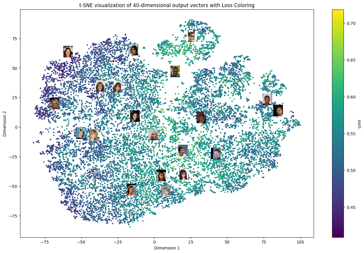
To visualize the statistical properties of the model’s outputs, we apply t-SNE to the final outputs of the wrapped model, projecting them into a two-dimensional space. In the resulting figure, we use vacuity loss values as a color map over the t-SNE feature space; brighter colors indicate higher vacuity loss, which corresponds to less typical images in the dataset. Additionally, we randomly select several data points and display their corresponding images near their positions on the plot.

# Apply t-SNE to reduce to 2 dimensions
tsne = TSNE(n_components=2, random_state=42)
tsne_result = tsne.fit_transform(output_vectors)

num_images = len(dataset_test)
# Randomly sample 20 indices from all images
np.random.seed(42)  # For reproducibility
sampled_indices = np.random.choice(num_images, 20, replace=False)

norm = plt.Normalize(vmin=losses.min(), vmax=losses.max())
cmap = cm.viridis

# Plot the t-SNE results with loss-based coloring
plt.figure(figsize=(16, 10))
sc = plt.scatter(tsne_result[:, 0], tsne_result[:, 1], c=losses, cmap=cmap, s=5, norm=norm)
plt.colorbar(sc, label='Loss')

# Function to add small images to the plot
def add_image(ax, image, xy):
    im = OffsetImage(image, zoom=0.1)
    ab = AnnotationBbox(im, xy, xybox=(20, 20), frameon=False, boxcoords="offset points", pad=0.3)
    ax.add_artist(ab)

# Add images at the specified indices
ax = plt.gca()
for idx in sampled_indices:
    add_image(ax, dataset_test[idx][0].cpu().numpy().transpose(1, 2, 0), tsne_result[idx])
plt.title('t-SNE visualization of 40-dimensional output vectors with Loss Coloring')
plt.xlabel('Dimension 1')
plt.ylabel('Dimension 2')
plt.show()

Plot Attribute Imbalance

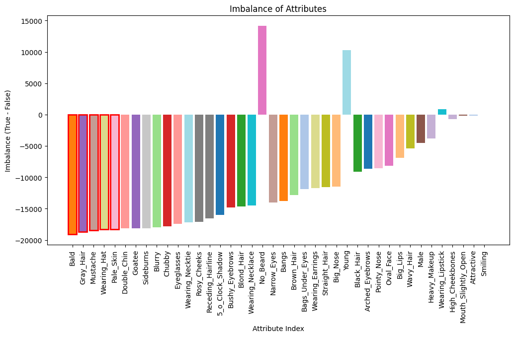
The dataset comprises 40 binary attributes, each labeled as either true or false. In the bar plot below, we display the imbalance for each attribute in the testing dataset, calculated as the number of true labels minus the number of false labels. The attributes are arranged in decreasing order of imbalance, so those with the highest imbalance appear first.

def load_attribute_names(file_path):
    with open(file_path, 'r') as f:
        lines = f.readlines()
    # The second line contains the attribute names
    attribute_names = lines[1].strip().split()
    return attribute_names

# Define the function to get the attribute values for a specific image index
def get_image_attributes(dataset, index):
    image, attributes = dataset[index]
    return image, attributes.numpy()

attr_file_path = os.path.join(CELEBA_DIR, 'labels', 'list_attr_celeba.txt')
attribute_names = load_attribute_names(attr_file_path)

# Calculate the imbalance for each attribute
imbalances = []
true_counts = []
false_counts = []
imbalances_ratio=[]
for attribute_index in range(40):
    true_count = np.sum(test_labels[:, attribute_index] == 1)
    false_count = np.sum(test_labels[:, attribute_index] == 0)
    imbalance = true_count - false_count
    imbalances_ratio.append((true_count/(true_count+false_count), attribute_index, attribute_names[attribute_index]))
    imbalances.append((imbalance, attribute_index, attribute_names[attribute_index]))

# Sort by imbalance and get the top 5 most unbalanced attributes
imbalances.sort(reverse=True, key=lambda x: abs(x[0]))
top_5_unbalanced = [idx for _, idx, _ in imbalances[:5]]

# Sort by imbalance
sorted_imbalances = [imb for imb, idx,_ in imbalances]
sorted_attributes = [idx for imb, _,idx in imbalances]
sorted_attributes_index = [idx for imb, idx,_ in imbalances]

# Plot the bar chart
plt.figure(figsize=(12, 6))
colors = cm.get_cmap('tab20', 40)
bars = plt.bar(range(40), sorted_imbalances, tick_label=sorted_attributes, color=[colors(i) for i in sorted_attributes_index])
# Highlight the top 5 most imbalanced attributes with red outlines
for i in range(5):
    bars[i].set_edgecolor('red')
    bars[i].set_linewidth(2)
plt.xticks(rotation=90)  # Rotate labels to be vertical
plt.xlabel('Attribute Index')
plt.ylabel('Imbalance (True - False)')
plt.title('Imbalance of Attributes')
plt.show()

The code block below processes the testing results in preparation for the figure plotted in the next code block. We start by filtering the vacuity losses to a smaller range because only a few images have very large vacuity losses outside this range. By focusing on this smaller range that contains almost all the images, we simplify the histogram we will draw. We then divide the vacuity losses into 10 subranges and count the number of images in each subrange for the histogram to be plotted next. The rest of the code identifies, within each vacuity loss range, the attributes whose distributions differ the most from those in the full testing dataset.

# Set the desired value range for the losses
min_value = 0 
max_value = 0.1

# Filter the losses to include only those within the specified range
filtered_losses = [loss for loss in losses if min_value <= loss <= max_value]

# Number of bins
num_bins = 10
# Use numpy's histogram function to get counts and bins without plotting
counts, bins = np.histogram(filtered_losses, bins=num_bins)

# Assign each loss to a bin
bin_indices = np.digitize(losses, bins=bins[:-1], right=False)  # Bins are 1-indexed

# Initialize a list to hold labels for each bin
labels_per_bin = [[] for _ in range(num_bins)]

# Group labels by their corresponding bin
for idx, bin_idx in enumerate(bin_indices):
    bin_idx = bin_idx - 1  # Adjust bin index to start from 0
    labels_per_bin[bin_idx].append(true_labels[idx].cpu()[0])

# Calculate how the imbalances for each attribute in each bin differ from the full testing data
top_5_unbalanced_ratio_attribute_per_bin=[]
top_5_unbalanced_ratio_direction_attribute_per_bin=[]
for bin_idx in range(10):
    imbalances = []
    imbalances_ratio_diffs = []
    for attribute_index in range(40):
        true_count = np.sum(np.array(labels_per_bin[bin_idx])[:, attribute_index] == 1)
        false_count = np.sum(np.array(labels_per_bin[bin_idx])[:, attribute_index] == 0)
        imbalances_ratio_diff = abs(true_count/(true_count+false_count)-imbalances_ratio[attribute_index][0])
        imbalances_ratio_diff_direction = (true_count/(true_count+false_count)-imbalances_ratio[attribute_index][0])>0
        imbalances_ratio_diffs.append((imbalances_ratio_diff, imbalances_ratio_diff_direction, attribute_index, attribute_names[attribute_index]))

    imbalances_ratio_diffs.sort(reverse=True, key=lambda x: x[0])
    top_5_unbalanced_ratio_diff = [idx for _, _, idx, _ in imbalances_ratio_diffs[:5]]
    top_5_unbalanced_ratio_diff_direction = [idx for _, idx, _, _ in imbalances_ratio_diffs[:5]]
    top_5_unbalanced_ratio_diff_attribute= [attribute_names[i] for i in top_5_unbalanced_ratio_diff]
    top_5_unbalanced_ratio_attribute_per_bin.append(top_5_unbalanced_ratio_diff_attribute)
    top_5_unbalanced_ratio_direction_attribute_per_bin.append(top_5_unbalanced_ratio_diff_direction)

Associate Vacuity with Presence/Absence of Attributes

In the top figure below, we present a histogram of the vacuity losses to show their frequency distribution. For each bin in this histogram, we randomly sample four images and display them in the bottom figure. Above each bin, we indicate the top two attributes whose imbalances differ the most from those of the full dataset. A black font indicates the presence of an attribute, while a red font indicates the absence/inverse of the attribute. This figure demonstrates how the values of vacuity losses relate to specific attributes and provides examples of typical images for each range of vacuity losses.

# Function to get 4 images for a given bin range
def get_images_for_loss_range(bin_range, n_samples=4):
    bin_indices = [i for i, loss in enumerate(losses) if bin_range[0] <= loss < bin_range[1]]

    if len(bin_indices) < n_samples:
        n_samples = len(bin_indices)
    
    sampled_indices = np.random.choice(bin_indices, n_samples, replace=False)
    
    images = [dataset_test[i][0].permute(1, 2, 0).cpu().numpy() for i in sampled_indices]  # Convert to (H, W, C)
    
    return images

# Collect 4 images for each bin (within the filtered range)
images_per_bin = []
for i in range(num_bins):
    bin_range = (bins[i], bins[i+1])
    images = get_images_for_loss_range(bin_range)
    images_per_bin.append(images)

# Plot the histogram
plt.figure(figsize=(16, 8))
bin_width = (bins[1] - bins[0]) * 0.6
plt.bar(bins[:-1], counts, width=bin_width, edgecolor='black', align='edge')

# Add vertical dashed lines
for i in range(1, len(bins) - 1):
    plt.axvline(x=bins[i] - (bins[1] - bins[0]) * 0.2, color='gray', linestyle='--', linewidth=1)

# Determine the fixed y-coordinate for the additional texts
max_count = max(counts)
y_text_fixed = max_count +1000  # Adjust this value as needed

# Add text annotations
for i in range(len(counts)):
    bar_center = (bins[i] + bins[i+1]) / 2

    y_base = counts[i] + 0.5
    plt.text(bar_center, y_base, f'Bin {i+1}', ha='center', fontsize=10)

    texts = top_5_unbalanced_ratio_attribute_per_bin[i]
    directions = top_5_unbalanced_ratio_direction_attribute_per_bin[i]
    
    for j in range(2):
        text = texts[j]
        direction = directions[j]
        color = 'black' if direction else 'red'
        y_offset = y_text_fixed + j * 500
        plt.text(bar_center, y_offset, text, ha='center', fontsize=10, color=color)

plt.ylim(top=y_offset + 500)

plt.xlabel('Loss')
plt.ylabel('Count')
plt.title('Histogram with Text Annotations per Bin')

plt.show()

# Create a figure with 1 row and 10 columns for each 2x2 image grid
fig = plt.figure(figsize=(20, 4)) 

outer_grid = gridspec.GridSpec(1, 10, figure=fig, wspace=0.05, hspace=0)

for i, imgs in enumerate(images_per_bin):
    ax = plt.subplot(outer_grid[i])
    
    inner_grid = gridspec.GridSpecFromSubplotSpec(2, 2, subplot_spec=outer_grid[i], wspace=0, hspace=-0.58)
    
    for j, img in enumerate(imgs):
        ax2 = plt.Subplot(fig, inner_grid[j])
        ax2.imshow(img)
        ax2.axis('off')
        ax2.set_xticks([])
        ax2.set_yticks([])
        fig.add_subplot(ax2)

    ax.set_title(f'Bin {i+1}', fontsize=16, y=0.8)
    ax.axis('off') 

fig.suptitle('4 Images for Each Loss Bin (Filtered Range)', fontsize=16)
plt.tight_layout()
plt.subplots_adjust(wspace=0.05, hspace=0)  
plt.show()

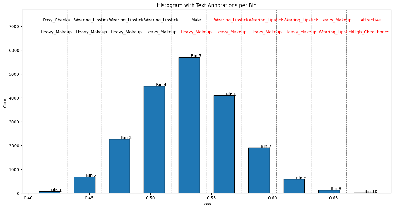
Based on the figure above, we observe that images with the smallest vacuity losses predominantly feature young women. Young men also appear frequently among images with low vacuity losses, particularly in Bins 2 and 3. As the vacuity loss increases beyond Bin 3, the images exhibit greater diversity, including individuals with darker skin tones, older adults, and people wearing accessories like glasses or hats.

Step 4: Resample Dataset to Reduce Bias

We can resample the testing dataset using sampling schemes that consider the vacuity losses of the images. A straightforward method is to sample images uniformly across bins defined by vacuity loss ranges. This involves two steps: first, we uniformly select a bin corresponding to a specific vacuity loss range; second, we randomly select an image from within that bin. This approach ensures that images from different vacuity loss ranges are equally represented in the resampled dataset.

import numpy as np
import torch
import matplotlib.pyplot as plt
import random

# Define a function to plot images in a 3x3 grid
def plot_images_grid(images, title):
    fig, axes = plt.subplots(3, 3, figsize=(8, 8))
    fig.suptitle(title, fontsize=16)
    
    for i, ax in enumerate(axes.flat):
        ax.imshow(images[i]) 
        ax.axis('off')
    
    plt.tight_layout()
    plt.show()

# 1. Uniform Random Sampling
n_samples = 9

uniform_indices = random.sample(range(len(dataset_test)), n_samples)

uniform_sampled_images = [dataset_test[i][0].permute(1, 2, 0) for i in uniform_indices]  # dataset_test[i] gives (image, label)

plot_images_grid(uniform_sampled_images, title='Uniformly Sampled Images')

# 2. Uniformly select 9 bins
uniform_bins = random.sample(range(num_bins), n_samples)

uniform_bins_sampled_images=[]
for i in uniform_bins:
    bin_range = (bins[i], bins[i+1])
    images = get_images_for_loss_range(bin_range,1)
    uniform_bins_sampled_images.append(images[0])

plot_images_grid(uniform_bins_sampled_images, title='Weighted Sampled Images Based on Vacuity Loss')

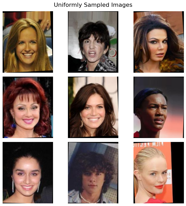
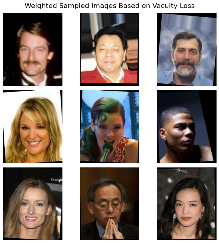
The example above demonstrates that the resampled images, guided by vacuity loss predictions from the wrapped model, exhibit greater diversity. Attributes such as wearing a hat, earrings, or glasses are also treated as factors contributing to the diversity of the dataset since they are included in the training labels.