Sample Wrapper: Generating MNIST Digits with DCGAN

In this tutorial we show how to wrap a Deep Convolutional Generative Adversarial Network (DCGAN) that generates images of handwritten digits with the Sample wrapper.

Generative Adversarial Networks (GANs) – two models are trained simultaneously by an adversarial process. A generator (“the artist”) learns to create images that look real, while a discriminator (“the art critic”) learns to tell real images apart from fakes.

During training, the generator progressively becomes better at creating images that look real, while the discriminator becomes better at telling them apart. The process reaches equilibrium when the discriminator can no longer distinguish real images from fakes.

Lastly, we wrap the model with Sample wrapper and display the risk of generated images.

We are building upon this notebook authored by Google and licensed under the Creative Commons Attribution 4.0 License, and code samples are licensed under the Apache 2.0 License. For details, see the Google Developers Site Policies.

Step 1: Initial Setup

import os
import glob
import time

import numpy as np
import matplotlib.pyplot as plt
import tensorflow as tf
from tensorflow.keras import layers
from IPython import display

Load the MNIST dataset

(train_images, train_labels), (_, _) = tf.keras.datasets.mnist.load_data()

train_images = train_images.reshape(train_images.shape[0], 28, 28, 1).astype('float32')
train_images = (train_images - 127.5) / 127.5  # Normalize the images to [-1, 1]

BUFFER_SIZE = 60000
BATCH_SIZE = 256
noise_dim = 100

# Batch and shuffle the data
train_dataset = tf.data.Dataset.from_tensor_slices(train_images).shuffle(BUFFER_SIZE).batch(BATCH_SIZE)

Step 2: Create a model

DCGAN model has two parts:

• The generator learns to generate plausible data. The generated instances become negative training examples for the discriminator.

• The discriminator learns to distinguish the generator’s fake data from real data. The discriminator penalizes the generator for producing implausible results.

from tensorflow.keras import layers

def make_generator_model():
    model = tf.keras.Sequential(name='generator')
    model.add(layers.Dense(7*7*256, use_bias=False, input_shape=(100,)))
    model.add(layers.BatchNormalization())
    model.add(layers.LeakyReLU())

    model.add(layers.Reshape((7, 7, 256)))

    model.add(layers.Conv2DTranspose(128, (5, 5), strides=(1, 1), padding='same', use_bias=False))
    model.add(layers.BatchNormalization())
    model.add(layers.LeakyReLU())

    model.add(layers.Conv2DTranspose(64, (5, 5), strides=(2, 2), padding='same', use_bias=False))
    model.add(layers.BatchNormalization())
    model.add(layers.LeakyReLU())

    model.add(layers.Conv2DTranspose(1, (5, 5), strides=(2, 2), padding='same', use_bias=False, activation='tanh'))

    return model

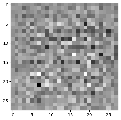
Use the (as yet untrained) generator to create an image.

noise = tf.random.normal([1, 100])
generator = make_generator_model()
generated_image = generator(noise, training=False)

plt.imshow(generated_image[0, :, :, 0], cmap='gray');

The discriminator is a CNN-based image classifier.

def make_discriminator_model():
    model = tf.keras.Sequential(name='discriminator')
    model.add(layers.Conv2D(64, (5, 5), strides=(2, 2), padding='same',
                                     input_shape=[28, 28, 1]))
    model.add(layers.LeakyReLU())

    model.add(layers.Conv2D(128, (5, 5), strides=(2, 2), padding='same'))
    model.add(layers.LeakyReLU())

    model.add(layers.Flatten())
    model.add(layers.Dense(1))

    return model

Use the (as yet untrained) discriminator to classify the generated images as real or fake. The model will be trained to output positive values for real images, and negative values for fake images.

discriminator = make_discriminator_model()
decision = discriminator(generated_image)
print(decision)

The generator’s loss quantifies how well it was able to trick the discriminator. Intuitively, if the generator is performing well, the discriminator will classify the fake images as real (or 1). Here, compare the discriminators decisions on the generated images to an array of 1s.

# This method returns a helper function to compute cross entropy loss
cross_entropy = tf.keras.losses.BinaryCrossentropy(from_logits=True)

def generator_loss(fake_output):
    return cross_entropy(tf.ones_like(fake_output), fake_output)

generator_optimizer = tf.optimizers.Adam(1e-4)

The discrimanator’s loss quantifies how well the discriminator is able to distinguish real images from fakes. It compares the discriminator’s predictions on real images to an array of 1s, and the discriminator’s predictions on fake (generated) images to an array of 0s.

def discriminator_loss(real_output, fake_output):
    real_loss = cross_entropy(tf.ones_like(real_output), real_output)
    fake_loss = cross_entropy(tf.zeros_like(fake_output), fake_output)
    total_loss = real_loss + fake_loss
    return total_loss

discriminator_optimizer = tf.optimizers.Adam(1e-4)

EPOCHS = 50
num_examples_to_generate = 16

seed = tf.random.normal([num_examples_to_generate, noise_dim])

Wrap the model with Sample wrapper

import capsa_tf

# NOTE: applying Capsa here

@capsa_tf.sample.Wrapper()
def wrapped_generator(noise, training=True):
    return generator(noise, training=training)

@tf.function
def forward_fn(noise, images):
    generated_images = wrapped_generator(noise, training=True)

    real_output = discriminator(images, training=True)
    fake_output = discriminator(generated_images, training=True)

    gen_loss = generator_loss(fake_output)
    disc_loss = discriminator_loss(real_output, fake_output)
    
    return generated_images, real_output, fake_output, gen_loss, disc_loss

@tf.function
def train_step(images):
    noise = tf.random.normal([BATCH_SIZE, noise_dim])

    with tf.GradientTape() as gen_tape, tf.GradientTape() as disc_tape:
        generated_images, real_output, fake_output, gen_loss, disc_loss = forward_fn(noise, images)

    # calling .trainable_variables on a Capsa wrapped model
    # returns a list of two elements, where:
    # - first element contains flat list of Capsa added variables
    # - second element contains flat list of original model variables
    capsa_vars, user_vars = wrapped_generator.trainable_variables
    # for convenience, unpack these variables into a single flat list
    wrapped_generator_variables = [*capsa_vars, *user_vars]

    # NOTE: compute gradient of gen_loss wrt all trainable_variables of the wrapped_generator
    # and update wrapped_generator's trainable_variables with the computed gradient
    gradients_of_wrapped_generator = gen_tape.gradient(gen_loss, wrapped_generator_variables)
    generator_optimizer.apply_gradients(zip(gradients_of_wrapped_generator, wrapped_generator_variables))

    gradients_of_discriminator = disc_tape.gradient(disc_loss, discriminator.trainable_variables)
    discriminator_optimizer.apply_gradients(zip(gradients_of_discriminator, discriminator.trainable_variables))

# call on inputs
noise = tf.random.normal([BATCH_SIZE, noise_dim])
image_batch = next(iter(train_dataset))
print(image_batch.shape)

generated_images, real_output, fake_output, gen_loss, disc_loss = forward_fn(noise, image_batch)

(256, 28, 28, 1)

Step 3: Train the model

Generate and save images

def generate_images(predictions,color='gray'):
  fig = plt.figure(figsize=(4, 4))

  for i in range(predictions.shape[0]):
      plt.subplot(4, 4, i+1)
      plt.imshow(predictions[i, :, :, 0] * 127.5 + 127.5, cmap=color)
      plt.axis('off')

  plt.show()

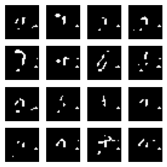
The training loop begins with generator receiving a random seed as input. That seed is used to produce an image. The discriminator is then used to classify real images (drawn from the training set) and fake images (produced by the generator). The loss is calculated for each of these models, and the gradients are used to update the generator and discriminator.

for epoch in range(EPOCHS):
    start = time.time()

    for image_batch in train_dataset:
      train_step(image_batch)

    display.clear_output(wait=True)
    predictions = generator(seed, training=False)
    generate_images(predictions)
    print ('Time for epoch {} is {} sec'.format(epoch + 1, time.time()-start))

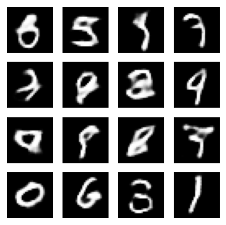
# Generate after the final epoch
display.clear_output(wait=True)
predictions = generator(seed, training=False)
generate_images(predictions)

Step 4: Visualize predictions & risk

# original function
output = generator(noise[:16])

# wrapped function outputs risk
output, risks = wrapped_generator(noise[:16], return_risk=True)
# risk has the same shape as the original output of the wrapped model
print(output.shape)
print(risks.shape)

(16, 28, 28, 1)
(16, 28, 28, 1)

Plot predictions:

generate_images(output)

Plot risk values:

generate_images(risks,color=plt.cm.jet)

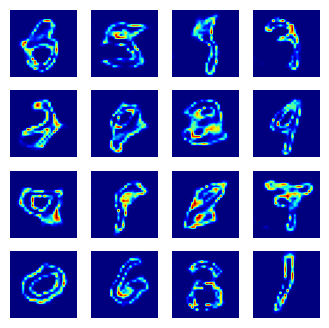
The risk of the generator model is higher for areas that do not appear frequently in the generation process, indicating they are less similar to handwritten digits.