Neo Wrapper: Image Classification with Out-of-Distribution Inputs

In this tutorial, we show how to wrap convolutional models with Neo wrapper, and visualize the vacuity loss.

The CIFAR-10 dataset is a widely-used benchmark dataset in machine learning, particularly for image classification tasks. It consists of 60,000 color images, each of size 32x32 pixels, spread across 10 different classes: airplanes, cars, birds, cats, deer, dogs, frogs, horses, ships, and trucks. The dataset is divided into 50,000 training images and 10,000 test images. CIFAR-10 is commonly used for evaluating the performance of classification algorithms due to its manageable size and diverse categories.

Step 1: Initial Setup and Wrapping

Import requirements

import argparse
import torch, torchvision
import torch.nn as nn
import torch.optim as optim
from torch.optim import lr_scheduler
import torchvision.datasets as datasets
import torch.utils.data as data
import torchvision.transforms as transforms
from torch.autograd import Variable
import torchvision.models as models
import matplotlib.pyplot as plt
import time, os, copy, numpy as np
import os
import gc
import torch.nn.functional as FTh
import torch.backends.cudnn as cudnn
from datetime import datetime
import torchvision
import sys 
from PIL import Image
from torch.utils.data import DataLoader
from sklearn.metrics import roc_curve, auc
from sklearn.decomposition import PCA
from torch.fx import symbolic_trace, Graph, GraphModule
import argparse
import os
import matplotlib.pyplot as plt
import logging
import sys
import math
device = torch.device("cuda:0")
torch.set_default_device(device)

Define and initialize the model

We can load various convolutional models that is pretrained on Cifar10, and wrap them. The pretrained model is from the pytorch-cifar-models repository. Here we provide an example that is cifar10_repvgg_a2, you can also wrap other models by changing the model name, examples including cifar10_resnet20, cifar10_resnet56 and cifar10_vgg19_bn. The full list of models can be found on the github page.

from capsa_torch import neo
def create_model(model_name, device):
    net = torch.hub.load("chenyaofo/pytorch-cifar-models", model_name, pretrained=True)

    net = net.to(device)
 
    wrapper=neo.Wrapper(integration_sites=2,layer_alpha=(2,1))

    wrapped_model=wrapper(net)
   

    wrapped_model = wrapped_model.to(device)

    logging.info(wrapped_model)
    return wrapped_model
model_name = "cifar10_repvgg_a2"
device = torch.device("cuda:0")
wrapped_model = create_model(model_name, device)

Step 2: Initialize Dataset

The model wrapped with the Neo Wrapper must be trained. In order to compare the vacuity scores, we divide the classes in the Cifar10 datasets as ID (in-distribution) and OOD (out-of-distribution), and we only train the model with ID data.

Augment CIFAR-10 Dataset with ID and OOD Class Labels

class FilteredCIFAR10(torchvision.datasets.CIFAR10):
    def __init__(self, root, train=True, transform=None, target_transform=None, download=False, id_classes=None, ood_classes=None):
        super().__init__(root, train=train, transform=transform, target_transform=target_transform, download=download)
        self.id_classes = id_classes
        self.ood_classes = ood_classes
        self.selected_indices = []
        self.id_ood_labels = []

        if self.id_classes is not None and self.ood_classes is not None:
            self.class_to_idx = {cls: idx for idx, cls in enumerate(self.classes)}
            for i, target in enumerate(self.targets):
                class_name = self.classes[target]
                if class_name in self.id_classes:
                    self.selected_indices.append(i)
                    self.id_ood_labels.append(0)  # 0 for ID
                elif class_name in self.ood_classes:
                    self.selected_indices.append(i)
                    self.id_ood_labels.append(1)  # 1 for OOD

            self.targets = [self.targets[i] for i in self.selected_indices]
            self.data = self.data[self.selected_indices]

    def __getitem__(self, index):
        img, target = self.data[index], self.targets[index]
        id_ood_label = self.id_ood_labels[index]

        img = Image.fromarray(img)

        if self.transform is not None:
            img = self.transform(img)

        if self.target_transform is not None:
            target = self.target_transform(target)

        return img, target, id_ood_label

Download and Configure Dataset

# Define transformations
transform_train = transforms.Compose([
    transforms.RandomCrop(32, padding=4),
    transforms.RandomHorizontalFlip(),
    transforms.ToTensor(),
    transforms.Normalize((0.4914, 0.4822, 0.4465), (0.2023, 0.1994, 0.2010)),
])

g = torch.Generator(device=device)


transform_test = transforms.Compose([
    transforms.ToTensor(),
    transforms.Normalize((0.4914, 0.4822, 0.4465), (0.2023, 0.1994, 0.2010)),
])


# Load the full CIFAR-10 training and test datasets
trainset = torchvision.datasets.CIFAR10(
    root='./data', train=True, download=True, transform=transform_train)

# Define filtered dataset for ID and OOD classes
ood_classes = ['airplane', 'automobile', 'bird', 'cat']
id_classes = ['deer', 'dog', 'frog', 'horse', 'ship', 'truck']

# Filtered dataset with only ID classes
ID_trainset = FilteredCIFAR10(root='./data', train=True, download=True, transform=transform_train, id_classes=id_classes, ood_classes=[])

# Use the full test set for evaluation
testset = FilteredCIFAR10(root='./data', train=False, download=True, transform=transform_test, id_classes=id_classes, ood_classes=ood_classes)

# DataLoader for filtered datasets
trainloader = DataLoader(ID_trainset, batch_size=100, shuffle=True, num_workers=0, generator=g)
testloader = DataLoader(testset, batch_size=100, shuffle=False, num_workers=0, generator=g)

print(f"train dataset size: {len(trainset)}")

print(f"Filtered train dataset size (ID only): {len(ID_trainset)}")
print(f"Filtered test dataset size (ID + OOD): {len(testset)}")
logging.info(f"train dataset size: {len(trainset)}")

logging.info(f"Filtered train dataset size (ID only): {len(ID_trainset)}")
logging.info(f"Filtered test dataset size (ID + OOD): {len(testset)}")

Files already downloaded and verified
Files already downloaded and verified
Files already downloaded and verified
train dataset size: 50000
Filtered train dataset size (ID only): 30000
Filtered test dataset size (ID + OOD): 10000

Step 3: Train Model

Here we provide the training function to train the wrapped model.

def evaluate_model(model, dataloaders, device='cuda:0'):
    model.eval()
    with torch.no_grad():
        for inputs, labels, _ in dataloaders:
            inputs = inputs.to(device)
            labels = labels.to(device)
            output, risk=model(inputs, return_risk=True)

def train_wrapper(model_name, model, train_loader, val_loader, dataset_sizes, optimizer, scheduler, num_epochs=25, patience=5):
    device = torch.device("cuda:0" if torch.cuda.is_available() else "cpu")
    since = time.time()
    best_model_wts = copy.deepcopy(model.state_dict())
    best_loss = float('inf')

    train_losses = []
    val_losses = []

    patience_counter = 0

    for epoch in range(num_epochs):
        print('Epoch {}/{}'.format(epoch + 1, num_epochs))
        print('-' * 10)
        logging.info('Epoch {}/{}'.format(epoch + 1, num_epochs))
        logging.info('-' * 10)
        model.train()
        running_loss = 0.0

        for i, (inputs, labels, id_ood) in enumerate(train_loader):
            inputs = inputs.to(device)
            labels = labels.to(device)
            optimizer.zero_grad()
            output, risk =model(inputs, return_risk=True)
            loss = risk.mean()
            loss.backward()
            optimizer.step()

            # Statistics
            running_loss += loss.item() * inputs.size(0)
            print("\rTrain Iteration: {}/{}, Loss: {}.".format(i + 1, len(train_loader), loss.item() * inputs.size(0)), end="")
            sys.stdout.flush()

        epoch_loss = running_loss / dataset_sizes['train']
        train_losses.append(epoch_loss)

        scheduler.step()

        # Validation phase
        model.eval()   # Set model to evaluate mode
        running_loss = 0.0

        with torch.no_grad():
            for i, (inputs, labels, id_ood) in enumerate(val_loader):
                inputs = inputs.to(device)
                labels = labels.to(device)

                # Forward pass
                output, risk=model(inputs, return_risk=True)
                loss = risk.mean()

                # Statistics
                running_loss += loss.item() * inputs.size(0)
                print("\rVal Iteration: {}/{}, Loss: {}.".format(i + 1, len(val_loader), loss.item() * inputs.size(0)), end="")
                sys.stdout.flush()

        epoch_val_loss = running_loss / dataset_sizes['val']
        val_losses.append(epoch_val_loss)

        # Deep copy the model
        if epoch_val_loss < best_loss:
            best_loss = epoch_val_loss
            best_model_wts = copy.deepcopy(model.state_dict())
            patience_counter = 0  # Reset the patience counter
        else:
            patience_counter += 1

        # Early stopping check
        if patience_counter >= patience:
            print(f"Early stopping at epoch {epoch + 1}")
            logging.info(f"Early stopping at epoch {epoch + 1}")
            break

        # Print the metrics
        print()
        print('Train Loss: {:.4f}'.format(train_losses[-1]))
        print('Val Loss: {:.4f}'.format(val_losses[-1]))
        print()
        logging.info('Train Loss: {:.4f}'.format(train_losses[-1]))
        logging.info('Val Loss: {:.4f}'.format(val_losses[-1]))

    time_elapsed = time.time() - since
    print('Training complete in {:.0f}m {:.0f}s'.format(
        time_elapsed // 60, time_elapsed % 60))
    print('Best val Loss: {:4f}'.format(best_loss))
    logging.info('Training complete in {:.0f}m {:.0f}s'.format(
        time_elapsed // 60, time_elapsed % 60))
    logging.info('Best val Loss: {:4f}'.format(best_loss))

    # Load best model weights
    model.load_state_dict(best_model_wts)

    # Create the directory if it doesn't exist
    directory = os.path.join('wrapped_models', model_name)
    if not os.path.exists(directory):
        os.makedirs(directory)
    timestamp = datetime.now().strftime('%Y%m%d_%H%M%S')
    # Save the best model weights
    torch.save(model.state_dict(), os.path.join(directory, f"best_model_{timestamp}.pth"))
    
    # Plot the train and validation losses
    plt.figure(figsize=(10, 5))
    plt.plot(train_losses, label='Training Loss')
    plt.plot(val_losses, label='Validation Loss')
    plt.xlabel('Epoch')
    plt.ylabel('Loss')
    plt.legend()
    plt.title('Training and Validation Loss')
    lossplotname = os.path.join(directory, "training_loss.png")
    counter = 2
    while os.path.exists(lossplotname):
        lossplotname = os.path.join(directory, f"training_loss_{counter}.png")
        counter += 1
    plt.savefig(lossplotname)
    print(f"Figure saved to {lossplotname}")
    logging.info(f"Figure saved to {lossplotname}")
    plt.show()
    plt.close()

    return model, best_loss
# before setting up the parameter and training the model, we need to evaluate the model first to make show it wrapped
evaluate_model(wrapped_model, testloader)
# Observe that all parameters are being optimized
optimizer = optim.SGD(wrapped_model.parameters(), lr=0.0001, momentum=0.9)
# Decay LR by a factor of 0.1 every 7 epochs
exp_lr_scheduler = lr_scheduler.StepLR(optimizer, step_size=7, gamma=0.1)
wrapped_model, best_loss = train_wrapper(model_name, wrapped_model, trainloader, testloader, {'train':len(ID_trainset),'val':len(testset)}, optimizer, exp_lr_scheduler,
                       num_epochs=50)

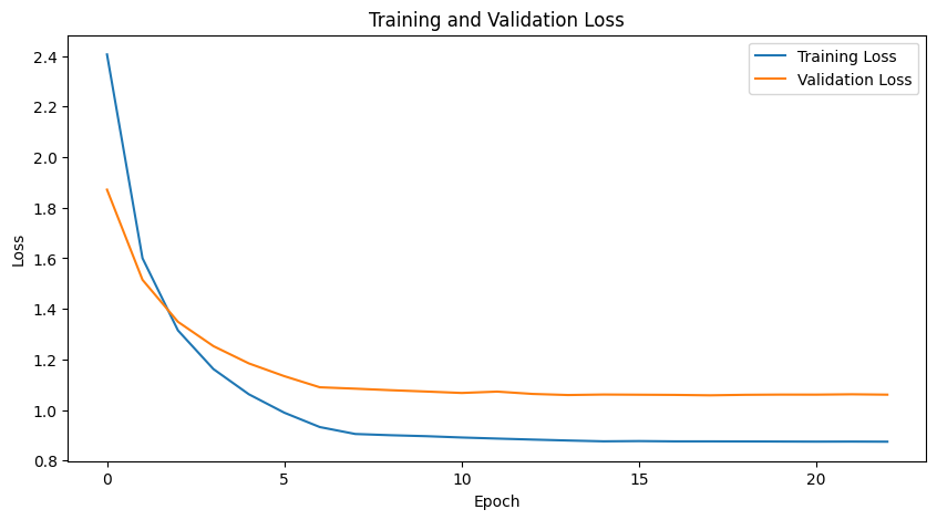
Epoch 1/50
----------
Val Iteration: 100/100, Loss: 187.62825727462769...
Train Loss: 2.4061
Val Loss: 1.8713

Epoch 2/50
----------
Val Iteration: 100/100, Loss: 151.93384885787964.5.
Train Loss: 1.6002
Val Loss: 1.5148

Epoch 3/50
----------
Val Iteration: 100/100, Loss: 135.6319546699524.68.
Train Loss: 1.3146
Val Loss: 1.3486

Epoch 4/50
----------
Val Iteration: 100/100, Loss: 126.15607976913452.5.
Train Loss: 1.1617
Val Loss: 1.2524

Epoch 5/50
----------
Val Iteration: 100/100, Loss: 119.14792060852051.5.
Train Loss: 1.0619
Val Loss: 1.1840

Epoch 6/50
----------
Val Iteration: 100/100, Loss: 113.99025917053223...
Train Loss: 0.9890
Val Loss: 1.1336

Epoch 7/50
----------
Val Iteration: 100/100, Loss: 109.83908176422119..
Train Loss: 0.9323
Val Loss: 1.0896

Epoch 8/50
----------
Val Iteration: 100/100, Loss: 109.19891595840454..
Train Loss: 0.9049
Val Loss: 1.0841

Epoch 9/50
----------
Val Iteration: 100/100, Loss: 108.64747762680054..
Train Loss: 0.9000
Val Loss: 1.0781

Epoch 10/50
----------
Val Iteration: 100/100, Loss: 108.07896852493286..
Train Loss: 0.8962
Val Loss: 1.0728

Epoch 11/50
----------
Val Iteration: 100/100, Loss: 107.73323774337769..
Train Loss: 0.8910
Val Loss: 1.0672

Epoch 12/50
----------
Val Iteration: 100/100, Loss: 107.90585279464722..
Train Loss: 0.8868
Val Loss: 1.0725

Epoch 13/50
----------
Val Iteration: 100/100, Loss: 107.21818208694458..
Train Loss: 0.8828
Val Loss: 1.0633

Epoch 14/50
----------
Val Iteration: 100/100, Loss: 106.64306879043579..
Train Loss: 0.8791
Val Loss: 1.0590

Epoch 15/50
----------
Val Iteration: 100/100, Loss: 106.94233179092407..
Train Loss: 0.8759
Val Loss: 1.0610

Epoch 16/50
----------
Val Iteration: 100/100, Loss: 106.96907043457031..
Train Loss: 0.8769
Val Loss: 1.0602

Epoch 17/50
----------
Val Iteration: 100/100, Loss: 106.92503452301025..
Train Loss: 0.8757
Val Loss: 1.0595

Epoch 18/50
----------
Val Iteration: 100/100, Loss: 106.77331686019897..
Train Loss: 0.8757
Val Loss: 1.0578

Epoch 19/50
----------
Val Iteration: 100/100, Loss: 106.93299770355225..
Train Loss: 0.8754
Val Loss: 1.0599

Epoch 20/50
----------
Val Iteration: 100/100, Loss: 107.05859661102295..
Train Loss: 0.8750
Val Loss: 1.0607

Epoch 21/50
----------
Val Iteration: 100/100, Loss: 106.98314905166626..
Train Loss: 0.8746
Val Loss: 1.0605

Epoch 22/50
----------
Val Iteration: 100/100, Loss: 107.06294775009155..
Train Loss: 0.8748
Val Loss: 1.0619

Epoch 23/50
----------
Val Iteration: 100/100, Loss: 107.08461999893188..Early stopping at epoch 23
Training complete in 24m 24s
Best val Loss: 1.057848
Figure saved to wrapped_models/cifar10_repvgg_a2/training_loss_5.png

Step 3: Evaluate Vacuity-Based ID/OOD Classification

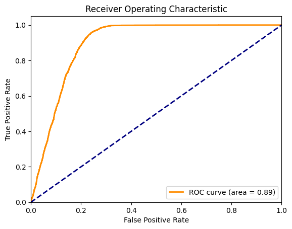
We added labels ID/OOD to the dataset, and as the vacuity score should reflect the type of uncertainty that arises from a lack of sufficient data or information, we expect higher vacuity scores for the OOD data. We can find a best threshold to divide the testing dataset into ID and OOD, and compare it with the true label. We plot the AUROC curve for this classification in order to evaluate its performance.

def evaluate_model(model, dataloaders, device='cuda:0'):
    model.eval()
    all_labels = []
    all_vacuity_scores = []
    all_id_ood_labels = []

    with torch.no_grad():
        for inputs, labels, id_ood_label in dataloaders:
            inputs = inputs.to(device)
            labels = labels.to(device)
            output, risk=model(inputs, return_risk=True)
            loss = risk.mean()
            all_labels.extend(labels.cpu().numpy())
            all_vacuity_scores.extend(risk.cpu().numpy())
            all_id_ood_labels.extend(id_ood_label.cpu().numpy())

    return np.array(all_labels), np.array(all_vacuity_scores), np.array(all_id_ood_labels)

def calculate_average_vacuity_scores(labels, vacuity_scores, id_ood_labels):
    labels = np.array(labels)
    vacuity_scores = np.array(vacuity_scores)
    id_ood_labels = np.array(id_ood_labels)
    
    # Separate the vacuity scores based on id_ood_labels
    vacuity_scores_id_0 = vacuity_scores[id_ood_labels == 0]
    vacuity_scores_id_1 = vacuity_scores[id_ood_labels == 1]
    
    # Calculate the average vacuity scores
    avg_vacuity_score_id_0 = np.mean(vacuity_scores_id_0)
    avg_vacuity_score_id_1 = np.mean(vacuity_scores_id_1)
    
    return avg_vacuity_score_id_0, avg_vacuity_score_id_1

def plot_roc_curve(model_name, id_ood_labels, vacuity_scores):
    fpr, tpr, thresholds = roc_curve(id_ood_labels, vacuity_scores)
    roc_auc = auc(fpr, tpr)

    # Plot ROC curve
    plt.figure()
    plt.plot(fpr, tpr, color='darkorange', lw=2, label='ROC curve (area = %0.2f)' % roc_auc)
    plt.plot([0, 1], [0, 1], color='navy', lw=2, linestyle='--')
    plt.xlim([0.0, 1.0])
    plt.ylim([0.0, 1.05])
    plt.xlabel('False Positive Rate')
    plt.ylabel('True Positive Rate')
    plt.title('Receiver Operating Characteristic')
    plt.legend(loc="lower right")
    directory = os.path.join('wrapped_models', model_name)
    if not os.path.exists(directory):
        os.makedirs(directory)
    plotname = os.path.join(directory, "roc_curve.png")
    base_plotname = plotname
    counter = 2
    while os.path.exists(plotname):
        plotname = os.path.join(directory, f"roc_curve_{counter}.png")
        counter += 1
    plt.savefig(plotname)
    plt.show()
    plt.close()

    return fpr, tpr, thresholds, roc_auc

labels, vacuity_scores, id_ood_labels=evaluate_model(wrapped_model,testloader)
avg_vacuity_score_id_0, avg_vacuity_score_id_1 = calculate_average_vacuity_scores(labels, vacuity_scores, id_ood_labels)
fpr, tpr, thresholds, roc_auc = plot_roc_curve(model_name, id_ood_labels, vacuity_scores)

Given the AUROC, the trained wrapped model evaluate a vacuity score that reflects the lack of sufficient data or information.

Additional Testing: Evaluating Other Models

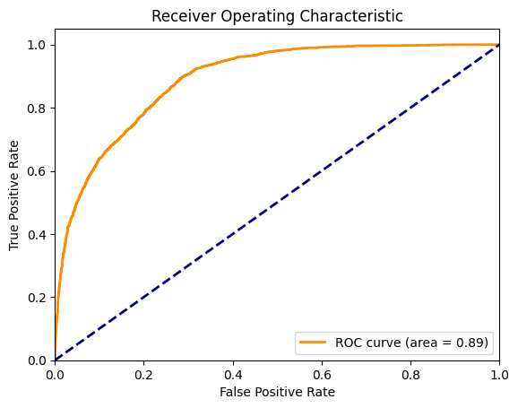
In addition to the model repvgg_a2, we can also wrap other models; here we provide an example using a ResNet20 classifier for CIFAR-10. You can change model_name to other such models like "cifar10_vgg19_bn" if you like.

# initialize model
model_name = "cifar10_resnet20"
device = torch.device("cuda:0")
wrapped_model = create_model(model_name, device)

# train the model
evaluate_model(wrapped_model, testloader) ## pass through sample inputs to the model before the training to finalize wrapping
optimizer = optim.SGD(wrapped_model.parameters(), lr=0.0001, momentum=0.9)
exp_lr_scheduler = lr_scheduler.StepLR(optimizer, step_size=7, gamma=0.1)
wrapped_model, best_loss = train_wrapper(model_name, wrapped_model, trainloader, testloader, {'train':len(ID_trainset),'val':len(testset)}, optimizer, exp_lr_scheduler,
                       num_epochs=50)

Using cache found in /home/liut6149/.cache/torch/hub/chenyaofo_pytorch-cifar-models_master

Epoch 1/50
----------
Val Iteration: 100/100, Loss: 179.0692687034607.46.
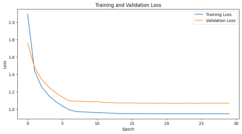
Train Loss: 2.0945
Val Loss: 1.7588

Epoch 2/50
----------
Val Iteration: 100/100, Loss: 150.62344074249268.8.
Train Loss: 1.4378
Val Loss: 1.4793

Epoch 3/50
----------
Val Iteration: 100/100, Loss: 136.9529128074646.38.
Train Loss: 1.2568
Val Loss: 1.3442

Epoch 4/50
----------
Val Iteration: 100/100, Loss: 128.10184955596924.8.
Train Loss: 1.1591
Val Loss: 1.2574

Epoch 5/50
----------
Val Iteration: 100/100, Loss: 121.2843656539917.35.
Train Loss: 1.0891
Val Loss: 1.1903

Epoch 6/50
----------
Val Iteration: 100/100, Loss: 115.95637798309326.3.
Train Loss: 1.0355
Val Loss: 1.1382

Epoch 7/50
----------
Val Iteration: 100/100, Loss: 111.51797771453857...
Train Loss: 0.9921
Val Loss: 1.0943

Epoch 8/50
----------
Val Iteration: 100/100, Loss: 111.30279302597046..
Train Loss: 0.9714
Val Loss: 1.0923

Epoch 9/50
----------
Val Iteration: 100/100, Loss: 110.93178987503052..
Train Loss: 0.9677
Val Loss: 1.0893

Epoch 10/50
----------
Val Iteration: 100/100, Loss: 110.41446924209595..
Train Loss: 0.9640
Val Loss: 1.0842

Epoch 11/50
----------
Val Iteration: 100/100, Loss: 110.67233085632324..
Train Loss: 0.9606
Val Loss: 1.0867

Epoch 12/50
----------
Val Iteration: 100/100, Loss: 109.81242656707764..
Train Loss: 0.9570
Val Loss: 1.0776

Epoch 13/50
----------
Val Iteration: 100/100, Loss: 109.40532684326172..
Train Loss: 0.9535
Val Loss: 1.0742

Epoch 14/50
----------
Val Iteration: 100/100, Loss: 109.11370515823364..
Train Loss: 0.9504
Val Loss: 1.0706

Epoch 15/50
----------
Val Iteration: 100/100, Loss: 109.0801477432251...
Train Loss: 0.9486
Val Loss: 1.0713

Epoch 16/50
----------
Val Iteration: 100/100, Loss: 109.15182828903198..
Train Loss: 0.9485
Val Loss: 1.0715

Epoch 17/50
----------
Val Iteration: 100/100, Loss: 108.79863500595093..
Train Loss: 0.9479
Val Loss: 1.0681

Epoch 18/50
----------
Val Iteration: 100/100, Loss: 108.86965990066528..
Train Loss: 0.9479
Val Loss: 1.0688

Epoch 19/50
----------
Val Iteration: 100/100, Loss: 108.84162187576294..
Train Loss: 0.9473
Val Loss: 1.0685

Epoch 20/50
----------
Val Iteration: 100/100, Loss: 108.82114171981812..
Train Loss: 0.9474
Val Loss: 1.0678

Epoch 21/50
----------
Val Iteration: 100/100, Loss: 108.96832942962646..
Train Loss: 0.9468
Val Loss: 1.0692

Epoch 22/50
----------
Val Iteration: 100/100, Loss: 108.72381925582886..
Train Loss: 0.9466
Val Loss: 1.0674

Epoch 23/50
----------
Val Iteration: 100/100, Loss: 108.647620677948....
Train Loss: 0.9467
Val Loss: 1.0666

Epoch 24/50
----------
Val Iteration: 100/100, Loss: 108.96118879318237..
Train Loss: 0.9463
Val Loss: 1.0695

Epoch 25/50
----------
Val Iteration: 100/100, Loss: 108.60106945037842..
Train Loss: 0.9467
Val Loss: 1.0660

Epoch 26/50
----------
Val Iteration: 100/100, Loss: 108.87913703918457..
Train Loss: 0.9460
Val Loss: 1.0688

Epoch 27/50
----------
Val Iteration: 100/100, Loss: 109.047532081604..3.
Train Loss: 0.9471
Val Loss: 1.0704

Epoch 28/50
----------
Val Iteration: 100/100, Loss: 108.74972343444824..
Train Loss: 0.9462
Val Loss: 1.0676

Epoch 29/50
----------
Val Iteration: 100/100, Loss: 109.079909324646..3.
Train Loss: 0.9465
Val Loss: 1.0697

Epoch 30/50
----------
Val Iteration: 100/100, Loss: 108.97228717803955..Early stopping at epoch 30
Training complete in 16m 47s
Best val Loss: 1.065991
Figure saved to wrapped_models/cifar10_resnet20/training_loss_3.png

labels, vacuity_scores, id_ood_labels=evaluate_model(wrapped_model,testloader)
avg_vacuity_score_id_0, avg_vacuity_score_id_1 = calculate_average_vacuity_scores(labels, vacuity_scores, id_ood_labels)
fpr, tpr, thresholds, roc_auc = plot_roc_curve(model_name, id_ood_labels, vacuity_scores)