Sample Wrapper: Regression

In this example, we will explore how to apply the Sample wrapper to regression data in order to identify epistemic risk, which arises from the predictive process. Epistemic risk quantifies the models understanding and confidence in its output.

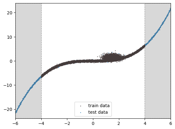
In the regression example below, we provide training data only within the range of -4 to 4, while the test data spans from -6 to 6. We will observe that the risk is higher in the regions -6 to -4 and 4 to 6, where training data is lacking. It is important to note that epistemic risk does not account for label noise, such as the noise in the training data between 0 to 2. To address this type of risk, we would need to consider aleatoric risk, which is demonstrated in our Sculpt wrapper.

Step 1: Imports and create data

import tensorflow as tf
import capsa_tf
import numpy as np
import numpy as np
import matplotlib.pyplot as plt

def plt_vspan(is_normalized=False):
    plt.axvspan(-6, -4, ec="black", color="grey", linestyle="--", alpha=0.3, zorder=3)
    plt.axvspan(4, 6, ec="black", color="grey", linestyle="--", alpha=0.3, zorder=3)
    if is_normalized:
        plt.xlim([-2, 2])
    else:
        plt.xlim([-6, 6])


def get_data(batch_size=256, is_shuffle=True, is_show=True):
    x = np.random.uniform(-4, 4, (16384, 1))
    x_val = np.linspace(-6, 6, 2048).reshape(-1, 1)

    y = x**3 / 10
    y_val = x_val**3 / 10

    # add noise to y
    y += np.random.normal(0, 0.2, (16384, 1))
    y_val += np.random.normal(0, 0.2, (2048, 1))

    # add greater noise in the middle to reproduce that plot from the 'Deep Evidential Regression' paper
    x = np.concatenate((x, np.random.normal(1.5, 0.3, 4096)[:, np.newaxis]), 0)
    y = np.concatenate((y, np.random.normal(1.5, 0.6, 4096)[:, np.newaxis]), 0)

    x_val = np.concatenate((x_val, np.random.normal(1.5, 0.3, 256)[:, np.newaxis]), 0)
    y_val = np.concatenate((y_val, np.random.normal(1.5, 0.6, 256)[:, np.newaxis]), 0)

    if is_shuffle:
        # otherwise loss increases in the beginning of each epoch
        # https://stackoverflow.com/questions/46928328/why-training-loss-is-increased-at-the-beginning-of-each-epoch

        train_shuffle_idx = np.arange(x.shape[0])
        np.random.shuffle(train_shuffle_idx)

        x = x[train_shuffle_idx]
        y = y[train_shuffle_idx]

    x, y, x_val, y_val = (
        x.astype(np.float32),
        y.astype(np.float32),
        x_val.astype(np.float32),
        y_val.astype(np.float32),
    )

    if is_show:
        plt.scatter(x, y, s=0.5, c="#463c3c", zorder=2, label="train data")
        plt.scatter(x_val, y_val, s=0.5, label="test data")
        plt_vspan()
        plt.legend()
        plt.show()

    return x, y, x_val, y_val

x_train, y_train, x_val, y_val = get_data(is_show=True)
x_batch, y_batch = x_train[:256], y_train[:256]
print(x_train.shape, y_train.shape)

(20480, 1) (20480, 1)

Step 2: Create and Wrap the model

initializer = tf.keras.initializers.GlorotNormal(seed=123)
W1 = tf.Variable(initializer(shape=(1, 8)))
W2 = tf.Variable(initializer(shape=(8, 16)))
W3 = tf.Variable(initializer(shape=(16, 16)))
W4 = tf.Variable(initializer(shape=(16, 1)))

initializer = tf.keras.initializers.Constant(0.05)
B1 = tf.Variable(initializer(shape=(8)))
B2 = tf.Variable(initializer(shape=(16)))
B3 = tf.Variable(initializer(shape=(16)))
B4 = tf.Variable(initializer(shape=(1)))

@capsa_tf.sample.Wrapper()
@tf.function
def fn(x):
    x = tf.matmul(x, W1) + B1
    x = tf.nn.relu(x)
    x = tf.matmul(x, W2) + B2
    x = tf.nn.relu(x)
    x = tf.matmul(x, W3) + B3
    x = tf.nn.relu(x)
    x = tf.matmul(x, W4) + B4
    return x

# simply calls on inputs
_ = fn(x_batch)

def loss_fn(x, y):
    y_hat = fn(x)
    loss = mse(y, y_hat)
    return loss, y_hat

mse = tf.losses.MeanSquaredError()

@tf.function
def train_step(x, y):
    
    with tf.GradientTape() as tape:
        loss, _ = loss_fn(x, y)

    trainable_vars = [W1, B1, W2, B2, W3, B3, W4, B4]
    gradients = tape.gradient(loss, trainable_vars)
    optimizer.apply_gradients(zip(gradients, trainable_vars))

    return loss


optimizer = tf.optimizers.Adam(learning_rate=0.0001)
train_step(x_batch, y_batch)

<tf.Tensor: shape=(), dtype=float32, numpy=1.255611>

Step 3: Train the Model

for ep in range(100):
    ep_loss = []
    for i in range(int(x_train.shape[0] // 256)):
        x_batch, y_batch = x_train[i*256:(i+1)*256], y_train[i*256:(i+1)*256]
        loss = train_step(x_batch, y_batch)
        ep_loss.append(loss)

Step 4: Visualize predictions & risk

def plot_2d(x_val, y_val, y_hat, risk=None):
    fig, axs = plt.subplots(2)
    axs[0].scatter(x_val, y_val, s=0.5, label="gt")
    axs[0].scatter(x_val, y_hat, s=0.5, label="yhat")
    plt_vspan()
    if risk is not None:
        axs[1].scatter(x_val, risk, s=0.5, label="epistemic")
    plt_vspan()
    plt.legend()
    plt.show()

y_hat, risk = fn(x_val, return_risk=True)
plot_2d(x_val, y_val, y_hat, risk)

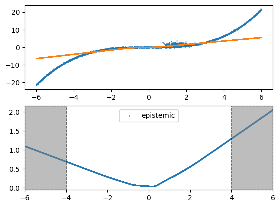
The result clearly indicates that epistemic risk is higher in areas lacking training data.