Vote Wrapper: MNIST Classification

In this tutorial we show how to wrap a MNIST classifier with the Vote wrapper. The Vote wrapper requires further training after the model wrapped, so we show here how to initialize and train the Vote wrapped model.

Step 1: Initial Setup

import torch
import torchvision
import torch.nn.functional as F
from torch.optim import Adam
import matplotlib.pyplot as plt
import tqdm

torch.manual_seed(1)
n_epochs = 5
batch_size = 128
learning_rate = 1e-3

Load the MNIST training and test set

train_loader = torch.utils.data.DataLoader(
    torchvision.datasets.MNIST(
        ".",
        train=True,
        download=True,
        transform=torchvision.transforms.Compose(
            [
                torchvision.transforms.ToTensor(),
                torchvision.transforms.Normalize((0.1307,), (0.3081,)),
            ]
        ),
    ),
    batch_size=batch_size,
    shuffle=True,
    drop_last=True,
)

test_loader = torch.utils.data.DataLoader(
    torchvision.datasets.MNIST(
        ".",
        train=False,
        download=True,
        transform=torchvision.transforms.Compose(
            [
                torchvision.transforms.ToTensor(),
                torchvision.transforms.Normalize((0.1307,), (0.3081,)),
            ]
        ),
    ),
    batch_size=batch_size,
    shuffle=True,
    drop_last=True,
)

Step 2: Define a model

In this tutorial we will use a simple convolutional neural network

class ConvMod(torch.nn.Module):
    def __init__(self):
        super().__init__()
        self.conv1 = torch.nn.Conv2d(1, 10, kernel_size=5)
        self.conv2 = torch.nn.Conv2d(10, 20, kernel_size=5)
        self.conv2_drop = torch.nn.Dropout2d()
        self.fc1 = torch.nn.Linear(320, 50)
        self.fc2 = torch.nn.Linear(50, 10)

    def forward(self, x):
        x = F.relu(F.max_pool2d(self.conv1(x), 2))
        x = F.relu(F.max_pool2d(self.conv2_drop(self.conv2(x)), 2))
        x = x.flatten(start_dim=1)
        x = F.relu(self.fc1(x))
        x = F.dropout(x)
        x = self.fc2(x)
        return x

model = ConvMod()

Step 3: Instantiate the wrapper and wrap the model

Here we create a new instance of the Vote wrapper with n_voters=8.

Then we wrap our model.

Since the Vote wrapper produces new parameters during wrapping, we need to trigger the wrapping process before instantiating our optimizer. To do so, simply call the wrapped model with sample inputs.

from capsa_torch import vote

wrapper = vote.Wrapper(n_voters=8)
model = wrapper(model)

sample_x, sample_y= next(iter(train_loader))
_ = model(sample_x)

Step 4: Training

Vote wrapper must be trained to in order to return accurate measures of uncertainty. Note that while training with the Vote wrapper in particular, you must pass tile_and_reduce=False to the wrapped model. You will also need to ensure that your batch_size is a multiple of n_voters. If you have an original trained model, the batch size after wrapping can be set to the number of voters times the original batch size.

model.train()
model.to('cuda')
optim = Adam(model.parameters(), lr=learning_rate)

for epoch in range(n_epochs):
    prog_bar = tqdm.tqdm(enumerate(train_loader), total=len(train_loader), postfix=dict(epoch=0, loss=0))

    for batch_idx, (x, y) in prog_bar:
        optim.zero_grad()
        pred= model(x.to('cuda'), training=True)
        loss = F.cross_entropy(pred, y.to('cuda'), reduction="mean")
        loss.backward()
        optim.step()

        prog_bar.set_postfix(epoch=epoch, loss=loss.item())

100%|██████████| 468/468 [00:10<00:00, 46.33it/s, epoch=0, loss=0.348]
100%|██████████| 468/468 [00:09<00:00, 49.73it/s, epoch=1, loss=0.227]
100%|██████████| 468/468 [00:09<00:00, 49.90it/s, epoch=2, loss=0.218] 
100%|██████████| 468/468 [00:09<00:00, 49.87it/s, epoch=3, loss=0.217] 
100%|██████████| 468/468 [00:09<00:00, 50.02it/s, epoch=4, loss=0.158] 

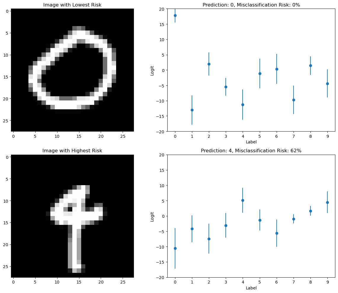
Step 5: Visualize and analysis the uncertainty

We visualize the images with smallest and largest uncertainties in the testing dataset, and plot the risks as error bars of the predictions for each label.

Note that for classification problems like this one, the capsa_torch interpret module provides a set of convenience functions to convert the risk scores produced by the Vote wrapper into interpretable quantities. For example, here we will use misclassification_prob_categorical to compute the probability that an input is misclassified.

# Move the model to CPU
model.to('cpu')

# Get a batch of test images and their labels
test_imgs, labels = next(iter(test_loader))

# Get predictions and risks for the test images
predictions, risk = model(test_imgs, training=False, return_risk=True)

# Calculate the average risk for each image
from capsa_torch.interpret import misclassification_prob_categorical
misclassification_risks = misclassification_prob_categorical(predictions, risk)

# Find the indices of the images with the smallest and largest average risk
min_risk_index = torch.argmin(misclassification_risks).item()
max_risk_index = torch.argmax(misclassification_risks).item()

# Plot the image with the smallest risk
fig, axes = plt.subplots(2, 2, figsize=(12, 10))

axes[0, 0].imshow(test_imgs[min_risk_index][0], cmap="gray")
axes[0, 0].set_title("Image with Lowest Risk")
axes[0, 1].errorbar(list(range(10)), predictions[min_risk_index].detach().numpy(), 
                    yerr=risk[min_risk_index].detach().numpy(), fmt='o')
axes[0, 1].set_ylabel('Logit')
axes[0, 1].set_ylim(-20, 20)
axes[0, 1].set_xticks(list(range(10)))
axes[0, 1].set_xlabel('Label')
axes[0, 1].set_title(f"Prediction: {torch.argmax(predictions[min_risk_index]).item()}, Misclassification Risk: {100*misclassification_risks[min_risk_index].item():.0f}%")

# Plot the image with the largest risk
axes[1, 0].imshow(test_imgs[max_risk_index][0], cmap="gray")
axes[1, 0].set_title("Image with Highest Risk")
axes[1, 1].errorbar(list(range(10)), predictions[max_risk_index].detach().numpy(), 
                    yerr=risk[max_risk_index].detach().numpy(), fmt='o')
axes[1, 1].set_ylabel('Logit')
axes[1, 1].set_ylim(-20, 20)
axes[1, 1].set_xticks(list(range(10)))
axes[1, 1].set_xlabel('Label')
axes[1, 1].set_title(f"Prediction: {torch.argmax(predictions[max_risk_index]).item()}, Misclassification Risk: {100*misclassification_risks[max_risk_index].item():.0f}%")

plt.tight_layout()
plt.show()